Download as PDF, PPTX


![Kruskal’s Algorithm
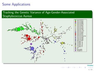
Algorithm
MST-KRUSKAL(G, w)
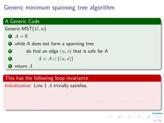
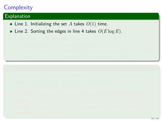
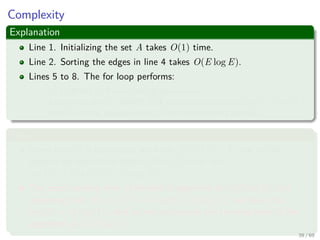
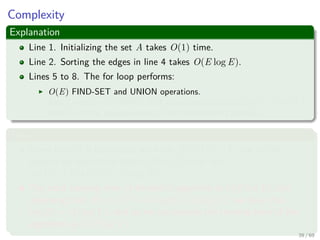
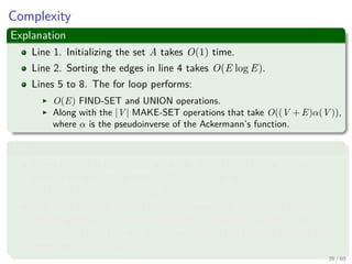
1 A = ∅
2 for each vertex v ∈ V [G]
3 do Make-Set
4 sort the edges of E into non-decreasing order by weight w
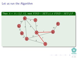
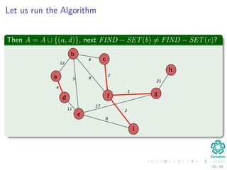
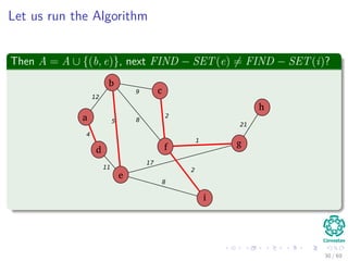
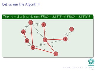
5 for each edge (u, v) ∈ E taken in non-decreasing order by weight
6 do if FIND − SET(u) = FIND − SET(v)
7 then A = A ∪ {(u, v)}
8 Union(u,v)
9 return A
22 / 69](https://image.slidesharecdn.com/19minimumspanningtrees-151108165156-lva1-app6891/85/19-Minimum-Spanning-Trees-36-320.jpg)
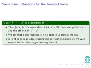
![Kruskal’s Algorithm
Algorithm
MST-KRUSKAL(G, w)
1 A = ∅
2 for each vertex v ∈ V [G]
3 do Make-Set
4 sort the edges of E into non-decreasing order by weight w
5 for each edge (u, v) ∈ E taken in non-decreasing order by weight
6 do if FIND − SET(u) = FIND − SET(v)
7 then A = A ∪ {(u, v)}
8 Union(u,v)
9 return A
22 / 69](https://image.slidesharecdn.com/19minimumspanningtrees-151108165156-lva1-app6891/85/19-Minimum-Spanning-Trees-37-320.jpg)
![Kruskal’s Algorithm
Algorithm
MST-KRUSKAL(G, w)
1 A = ∅
2 for each vertex v ∈ V [G]
3 do Make-Set
4 sort the edges of E into non-decreasing order by weight w
5 for each edge (u, v) ∈ E taken in non-decreasing order by weight
6 do if FIND − SET(u) = FIND − SET(v)
7 then A = A ∪ {(u, v)}
8 Union(u,v)
9 return A
22 / 69](https://image.slidesharecdn.com/19minimumspanningtrees-151108165156-lva1-app6891/85/19-Minimum-Spanning-Trees-38-320.jpg)
![Kruskal’s Algorithm
Algorithm
MST-KRUSKAL(G, w)
1 A = ∅
2 for each vertex v ∈ V [G]
3 do Make-Set
4 sort the edges of E into non-decreasing order by weight w
5 for each edge (u, v) ∈ E taken in non-decreasing order by weight
6 do if FIND − SET(u) = FIND − SET(v)
7 then A = A ∪ {(u, v)}
8 Union(u,v)
9 return A
22 / 69](https://image.slidesharecdn.com/19minimumspanningtrees-151108165156-lva1-app6891/85/19-Minimum-Spanning-Trees-39-320.jpg)


![Kruskal’s Algorithm
Algorithm
MST-KRUSKAL(G, w)
1 A = ∅
2 for each vertex v ∈ V [G]
3 do Make-Set
4 sort the edges of E into non-decreasing order by weight w
5 for each edge (u, v) ∈ E taken in non-decreasing order by weight
6 do if FIND − SET(u) = FIND − SET(v)
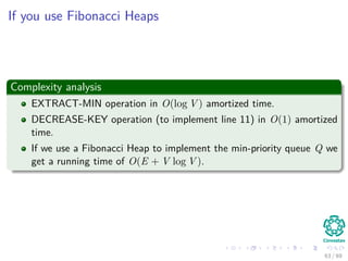
7 then A = A ∪ {(u, v)}
8 Union(u,v)
9 return A
38 / 69](https://image.slidesharecdn.com/19minimumspanningtrees-151108165156-lva1-app6891/85/19-Minimum-Spanning-Trees-55-320.jpg)

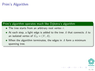
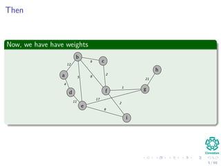
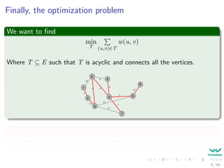
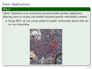
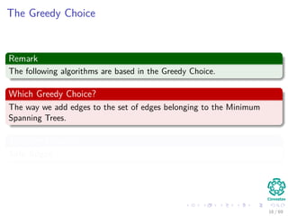
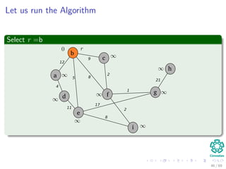
![The algorithm
Pseudo-code
MST-PRIM(G, w, r)
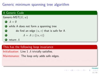
1 for each u ∈ V [G]
2 u.key = ∞
3 u.π = NIL
4 r.key = 0
5 Q = V [G]
6 while Q = ∅
7 u =Extract-Min(Q)
8 for each v ∈ Adj [u]
9 if v ∈ Q and w (u, v) < v.key
10 π [v] = u
11 v.key = w (u, v) an implicit decrease key
in Q
43 / 69](https://image.slidesharecdn.com/19minimumspanningtrees-151108165156-lva1-app6891/85/19-Minimum-Spanning-Trees-70-320.jpg)
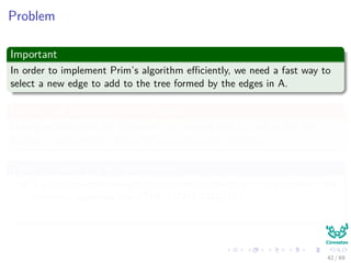
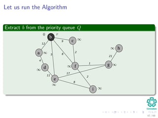
![The algorithm
Pseudo-code
MST-PRIM(G, w, r)
1 for each u ∈ V [G]
2 u.key = ∞
3 u.π = NIL
4 r.key = 0
5 Q = V [G]
6 while Q = ∅
7 u =Extract-Min(Q)
8 for each v ∈ Adj [u]
9 if v ∈ Q and w (u, v) < v.key
10 π [v] = u
11 v.key = w (u, v) an implicit decrease key
in Q
43 / 69](https://image.slidesharecdn.com/19minimumspanningtrees-151108165156-lva1-app6891/85/19-Minimum-Spanning-Trees-71-320.jpg)
![The algorithm
Pseudo-code
MST-PRIM(G, w, r)
1 for each u ∈ V [G]
2 u.key = ∞
3 u.π = NIL
4 r.key = 0
5 Q = V [G]
6 while Q = ∅
7 u =Extract-Min(Q)
8 for each v ∈ Adj [u]
9 if v ∈ Q and w (u, v) < v.key
10 π [v] = u
11 v.key = w (u, v) an implicit decrease key
in Q
43 / 69](https://image.slidesharecdn.com/19minimumspanningtrees-151108165156-lva1-app6891/85/19-Minimum-Spanning-Trees-72-320.jpg)
![The algorithm
Pseudo-code
MST-PRIM(G, w, r)
1 for each u ∈ V [G]
2 u.key = ∞
3 u.π = NIL
4 r.key = 0
5 Q = V [G]
6 while Q = ∅
7 u =Extract-Min(Q)
8 for each v ∈ Adj [u]
9 if v ∈ Q and w (u, v) < v.key
10 π [v] = u
11 v.key = w (u, v) an implicit decrease key
in Q
43 / 69](https://image.slidesharecdn.com/19minimumspanningtrees-151108165156-lva1-app6891/85/19-Minimum-Spanning-Trees-73-320.jpg)
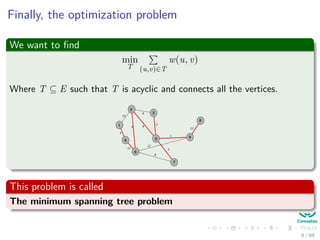
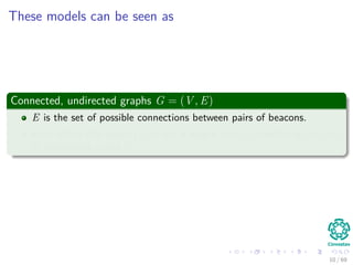
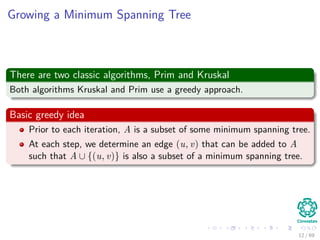
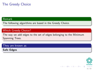
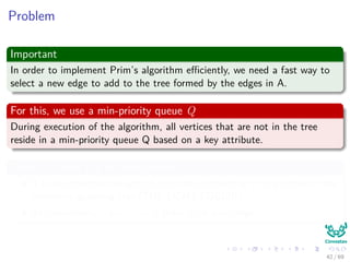
![Explanation
Observations
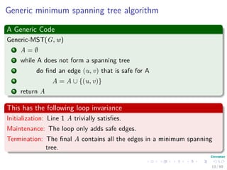
1 A = {(v, π[v]) : v ∈ V − {r} − Q}.
2 The vertices already placed into the minimum spanning tree are those
in V − Q.
3 For all vertices v ∈ Q, if π[v] = NIL, then key[v] < ∞ and key[v] is
the weight of a light edge (v, π[v]) connecting v to some vertex
already placed into the minimum spanning tree.
44 / 69](https://image.slidesharecdn.com/19minimumspanningtrees-151108165156-lva1-app6891/85/19-Minimum-Spanning-Trees-74-320.jpg)
![Explanation
Observations
1 A = {(v, π[v]) : v ∈ V − {r} − Q}.
2 The vertices already placed into the minimum spanning tree are those
in V − Q.
3 For all vertices v ∈ Q, if π[v] = NIL, then key[v] < ∞ and key[v] is
the weight of a light edge (v, π[v]) connecting v to some vertex
already placed into the minimum spanning tree.
44 / 69](https://image.slidesharecdn.com/19minimumspanningtrees-151108165156-lva1-app6891/85/19-Minimum-Spanning-Trees-75-320.jpg)
![Explanation
Observations
1 A = {(v, π[v]) : v ∈ V − {r} − Q}.
2 The vertices already placed into the minimum spanning tree are those
in V − Q.
3 For all vertices v ∈ Q, if π[v] = NIL, then key[v] < ∞ and key[v] is
the weight of a light edge (v, π[v]) connecting v to some vertex
already placed into the minimum spanning tree.
44 / 69](https://image.slidesharecdn.com/19minimumspanningtrees-151108165156-lva1-app6891/85/19-Minimum-Spanning-Trees-76-320.jpg)

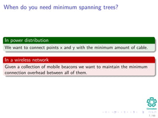
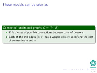
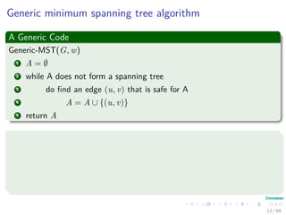
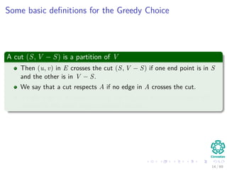
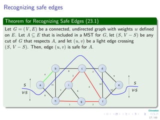
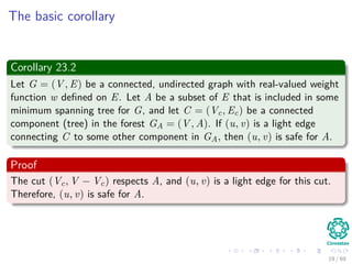
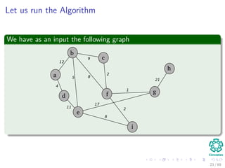
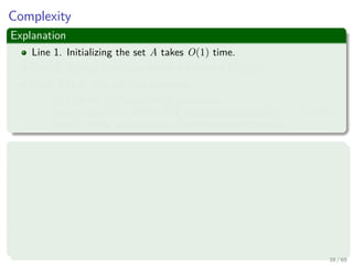
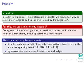
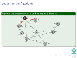
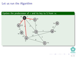
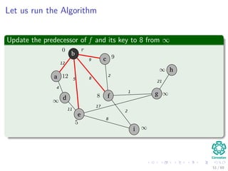
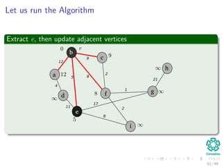
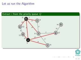
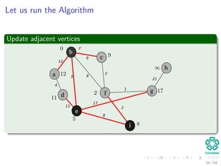
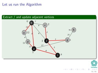
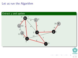
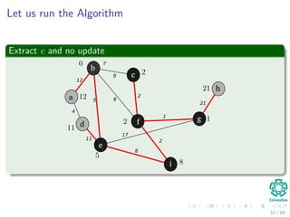
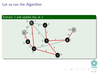
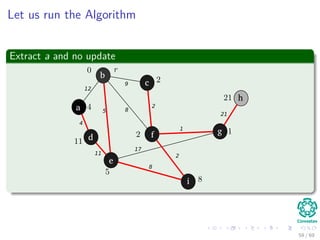
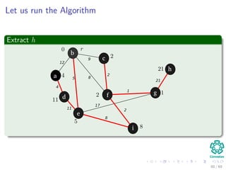
![Let us run the Algorithm
Update the predecessor of a and its key to 12 from ∞
b
c
f
a
d
e
i
g
h
12
4
5
11
8
9
2
1
17
8
2
21
Note: The RED color represent the field π [v]
48 / 69](https://image.slidesharecdn.com/19minimumspanningtrees-151108165156-lva1-app6891/85/19-Minimum-Spanning-Trees-80-320.jpg)


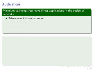
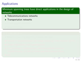
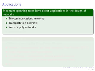
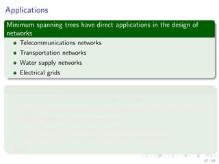
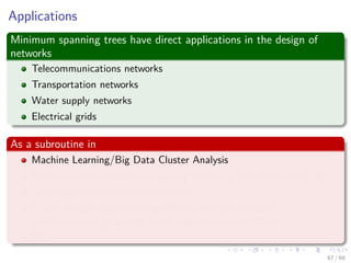


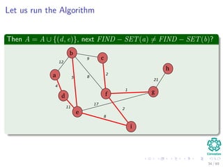
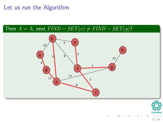
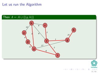
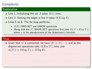
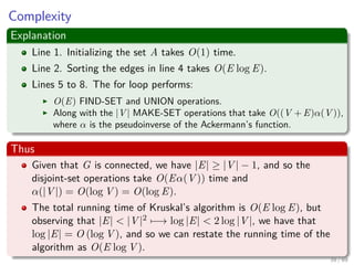
The document provides an overview of minimum spanning trees (MST) and algorithms associated with them, primarily Kruskal's and Prim's algorithms, which use a greedy approach to construct MSTs. It includes definitions of key concepts such as safe edges and cuts, the greedy choice principle, and situations where MSTs are applicable, such as in power distribution and wireless networks. Furthermore, it presents a generic MST algorithm and detailed steps for implementing Kruskal's algorithm.


![DAA-seminar-1[1].pptx Design and Analysis Of The Algorithm](https://cdn.slidesharecdn.com/ss_thumbnails/daa-seminar-11-250921155526-8ea0ea04-thumbnail.jpg?width=640&height=640&fit=bounds)