Download as PDF, PPTX


![Initialize and Relaxation
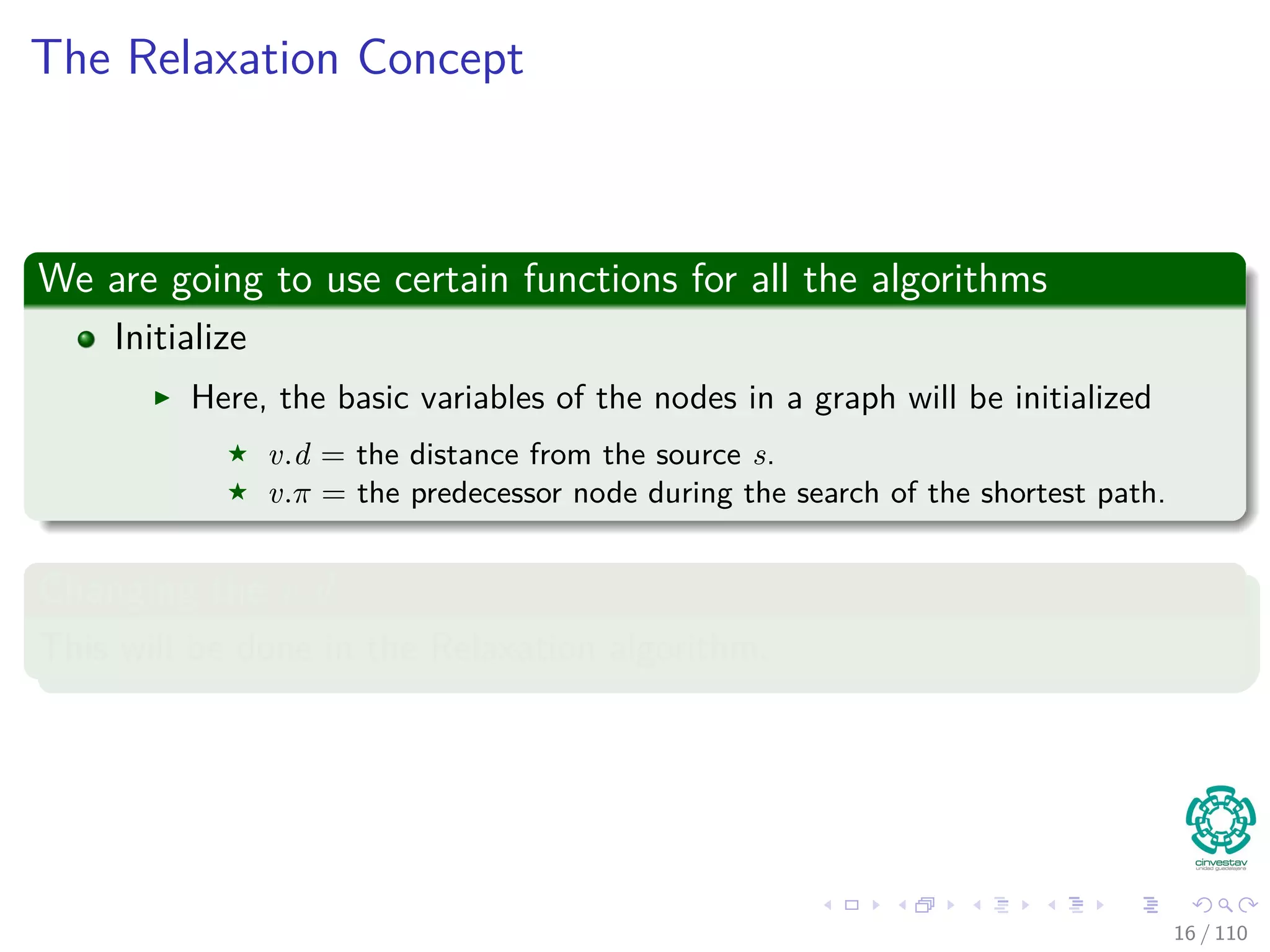
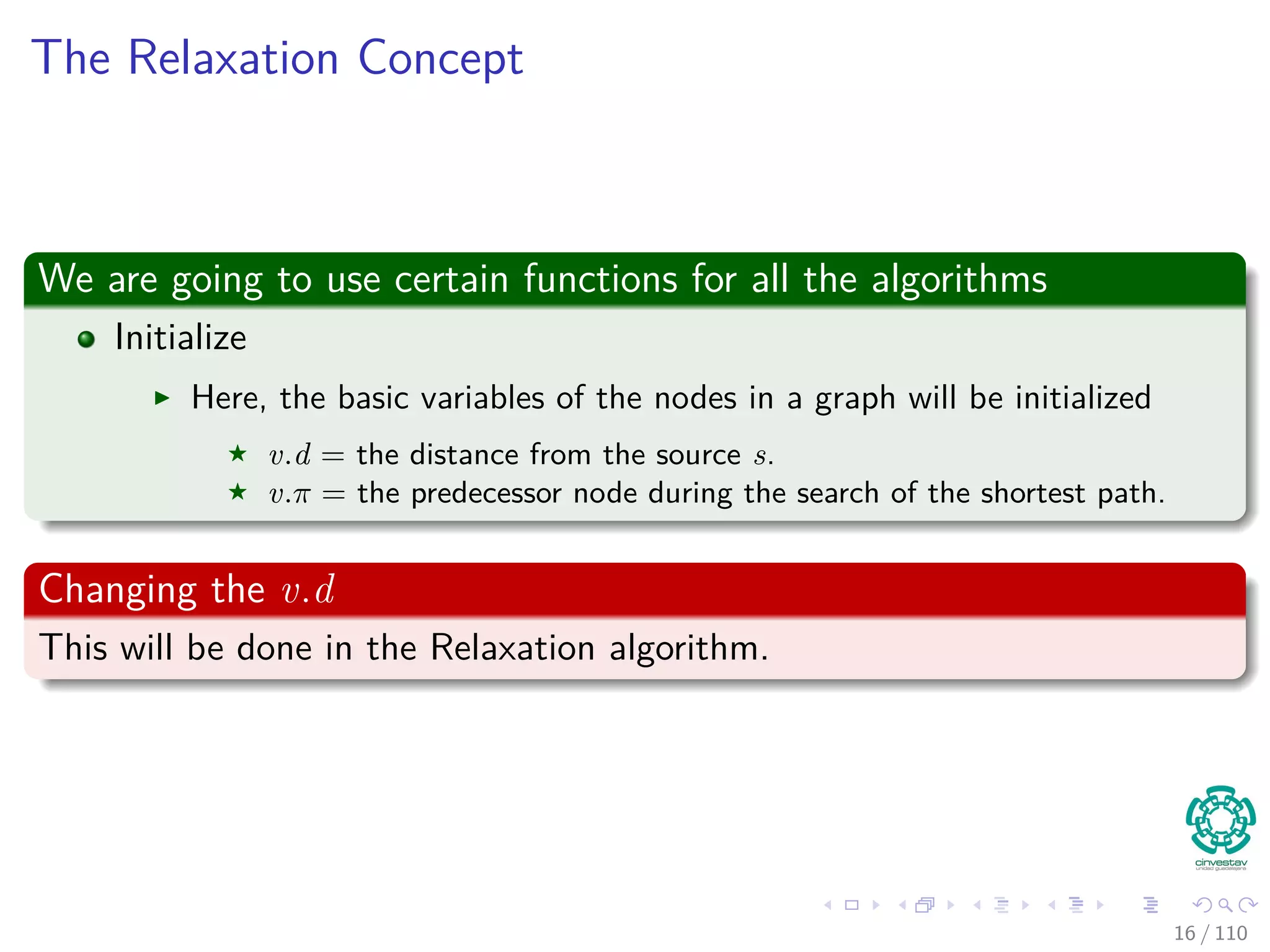
The Algorithms keep track of v.d, v.π. It is initialized as follows
Initialize(G, s)
1 for each v ∈ V [G]
2 v.d = ∞
3 v.π = NIL
4 s.d = 0
These values are changed when an edge (u, v) is relaxed.
Relax(u, v, w)
1 if v.d > u.d + w(u, v)
2 v.d = u.d + w(u, v)
3 v.π = u
17 / 108](https://image.slidesharecdn.com/20single-sourceshorthestpath-151109143432-lva1-app6891/75/20-Single-Source-Shorthest-Path-38-2048.jpg)
![Initialize and Relaxation
The Algorithms keep track of v.d, v.π. It is initialized as follows
Initialize(G, s)
1 for each v ∈ V [G]
2 v.d = ∞
3 v.π = NIL
4 s.d = 0
These values are changed when an edge (u, v) is relaxed.
Relax(u, v, w)
1 if v.d > u.d + w(u, v)
2 v.d = u.d + w(u, v)
3 v.π = u
17 / 108](https://image.slidesharecdn.com/20single-sourceshorthestpath-151109143432-lva1-app6891/75/20-Single-Source-Shorthest-Path-39-2048.jpg)

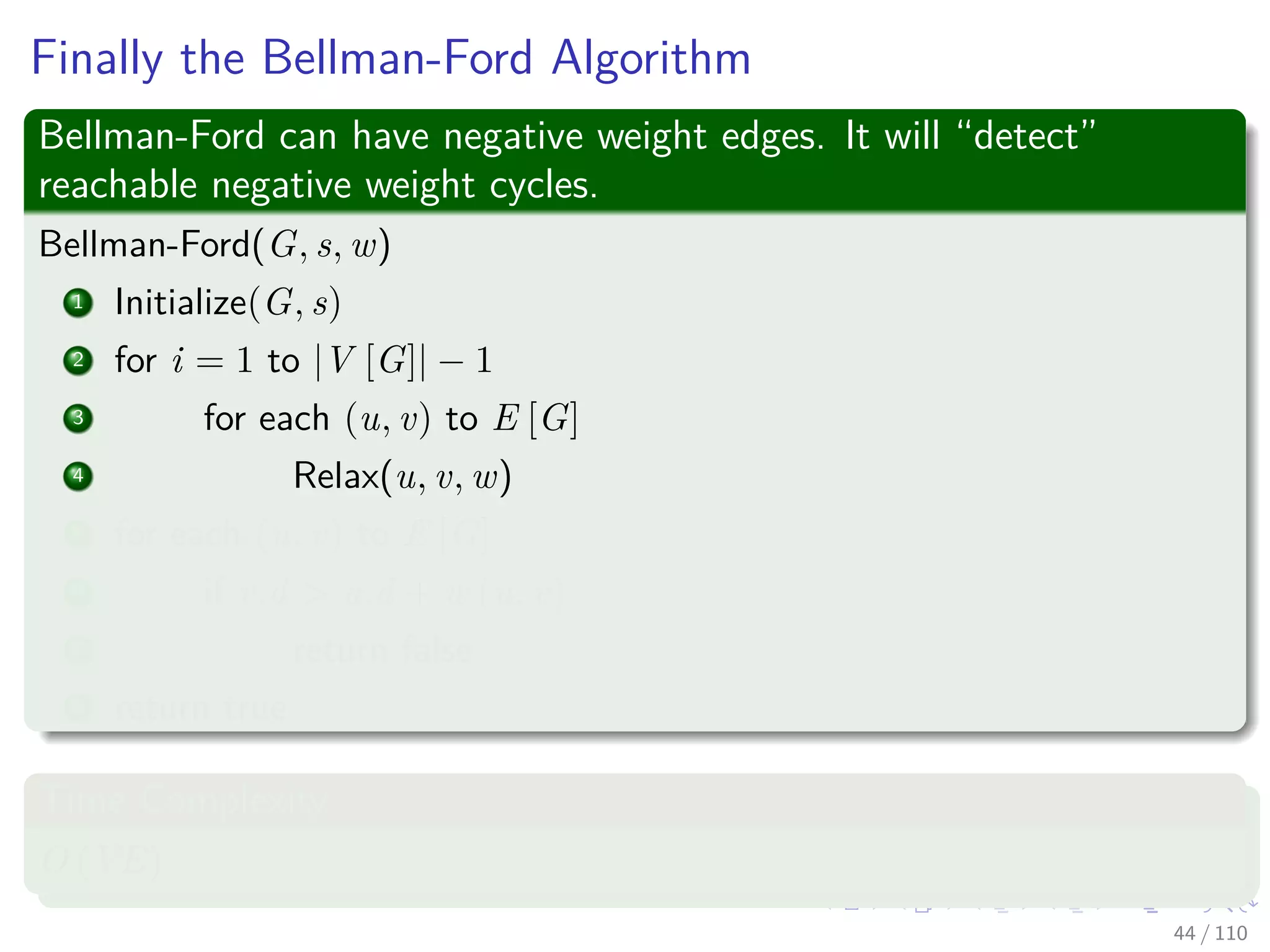
![The Bellman-Ford Algorithm
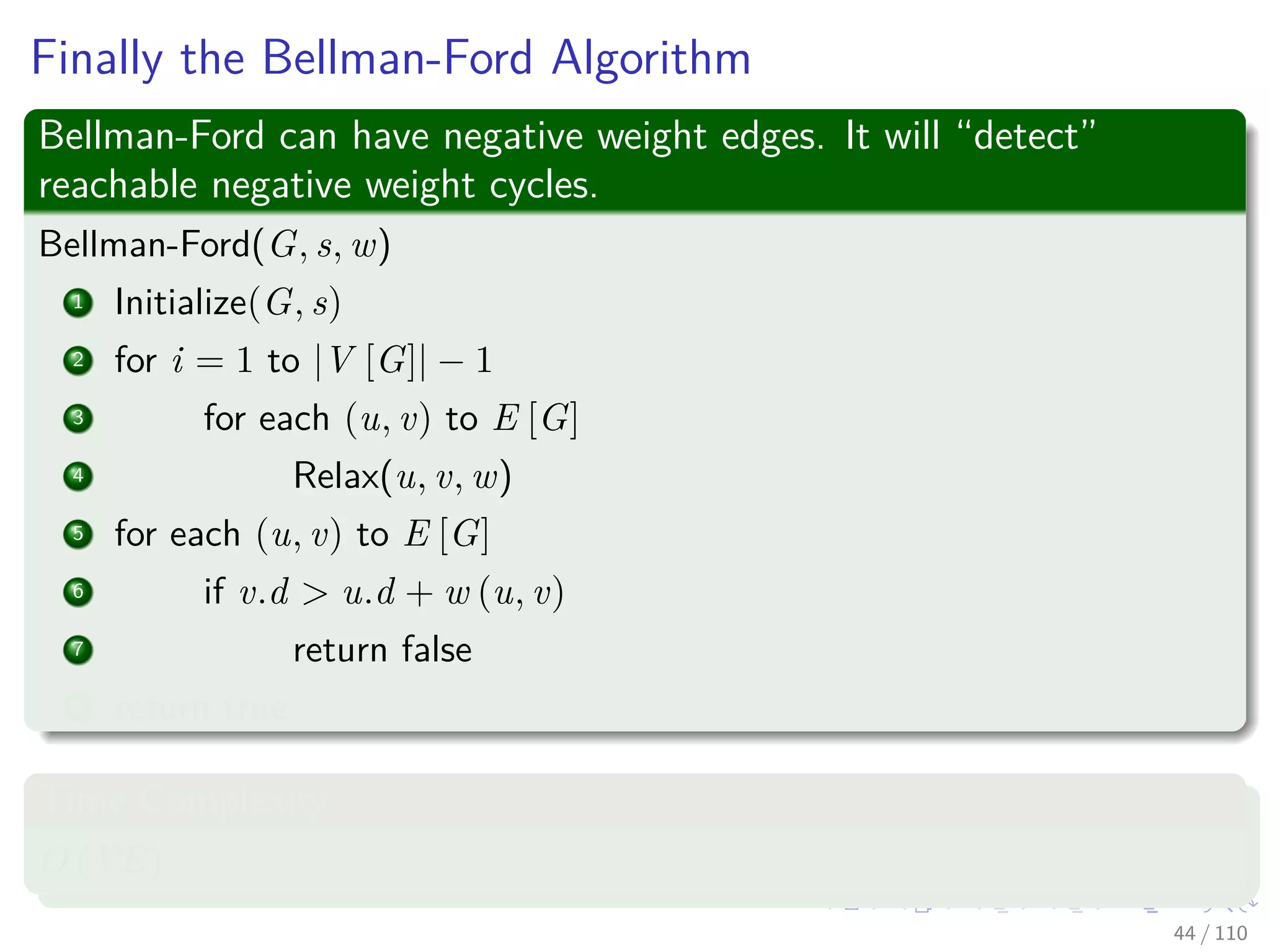
Bellman-Ford can have negative weight edges. It will “detect”
reachable negative weight cycles.
Bellman-Ford(G, s, w)
1 Initialize(G, s)
2 for i = 1 to |V [G]| − 1
3 for each (u, v) to E [G]
4 Relax(u, v, w)
5 for each (u, v) to E [G]
6 if v.d > u.d + w (u, v)
7 return false
8 return true
Time Complexity
O (VE)
20 / 108](https://image.slidesharecdn.com/20single-sourceshorthestpath-151109143432-lva1-app6891/75/20-Single-Source-Shorthest-Path-43-2048.jpg)
![The Bellman-Ford Algorithm
Bellman-Ford can have negative weight edges. It will “detect”
reachable negative weight cycles.
Bellman-Ford(G, s, w)
1 Initialize(G, s)
2 for i = 1 to |V [G]| − 1
3 for each (u, v) to E [G]
4 Relax(u, v, w)
5 for each (u, v) to E [G]
6 if v.d > u.d + w (u, v)
7 return false
8 return true
Time Complexity
O (VE)
20 / 108](https://image.slidesharecdn.com/20single-sourceshorthestpath-151109143432-lva1-app6891/75/20-Single-Source-Shorthest-Path-44-2048.jpg)
![The Bellman-Ford Algorithm
Bellman-Ford can have negative weight edges. It will “detect”
reachable negative weight cycles.
Bellman-Ford(G, s, w)
1 Initialize(G, s)
2 for i = 1 to |V [G]| − 1
3 for each (u, v) to E [G]
4 Relax(u, v, w)
5 for each (u, v) to E [G]
6 if v.d > u.d + w (u, v)
7 return false
8 return true
Time Complexity
O (VE)
20 / 108](https://image.slidesharecdn.com/20single-sourceshorthestpath-151109143432-lva1-app6891/75/20-Single-Source-Shorthest-Path-45-2048.jpg)
![The Bellman-Ford Algorithm
Bellman-Ford can have negative weight edges. It will “detect”
reachable negative weight cycles.
Bellman-Ford(G, s, w)
1 Initialize(G, s)
2 for i = 1 to |V [G]| − 1
3 for each (u, v) to E [G]
4 Relax(u, v, w)
5 for each (u, v) to E [G]
6 if v.d > u.d + w (u, v)
7 return false
8 return true
Time Complexity
O (VE)
20 / 108](https://image.slidesharecdn.com/20single-sourceshorthestpath-151109143432-lva1-app6891/75/20-Single-Source-Shorthest-Path-46-2048.jpg)


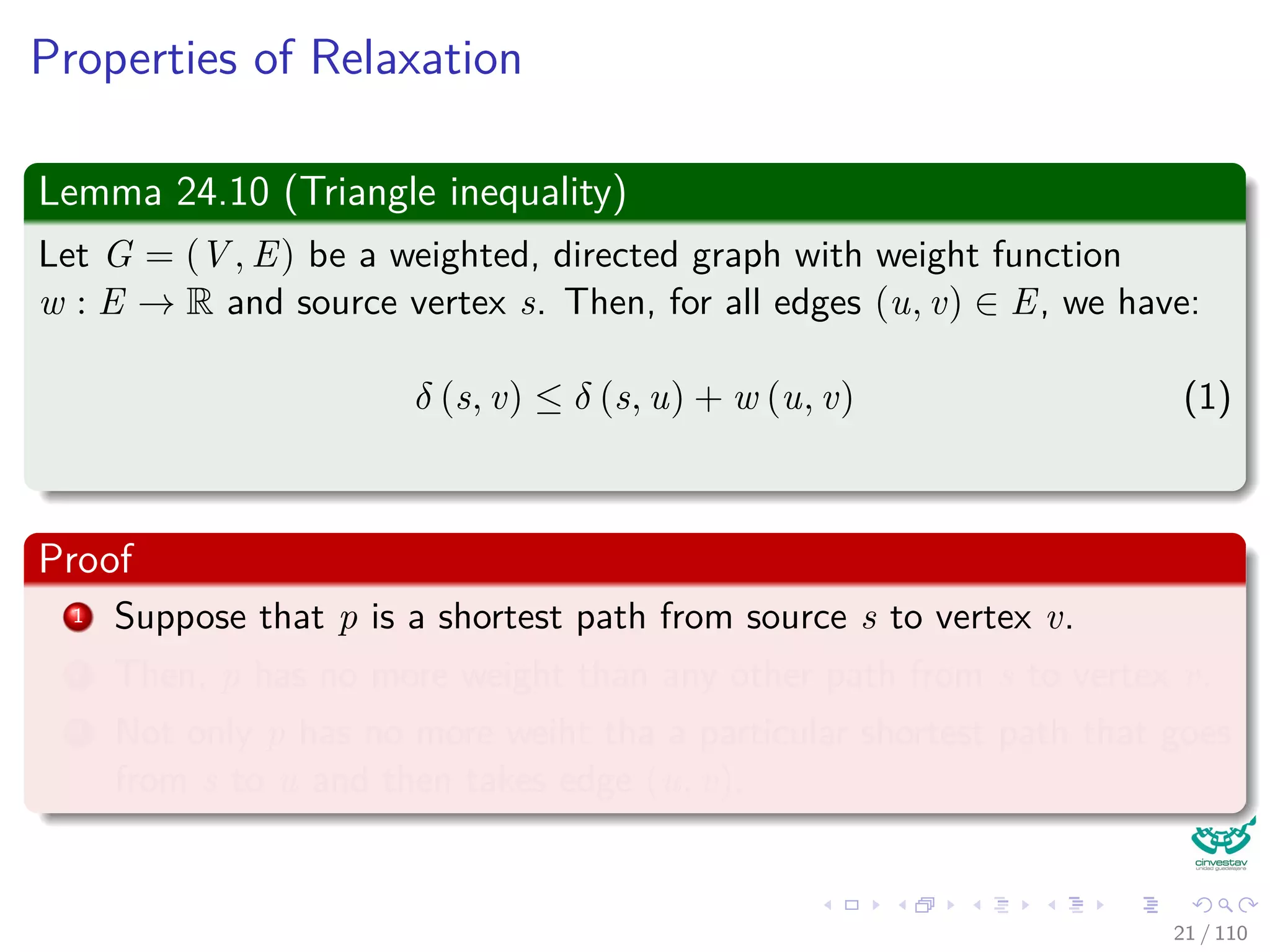
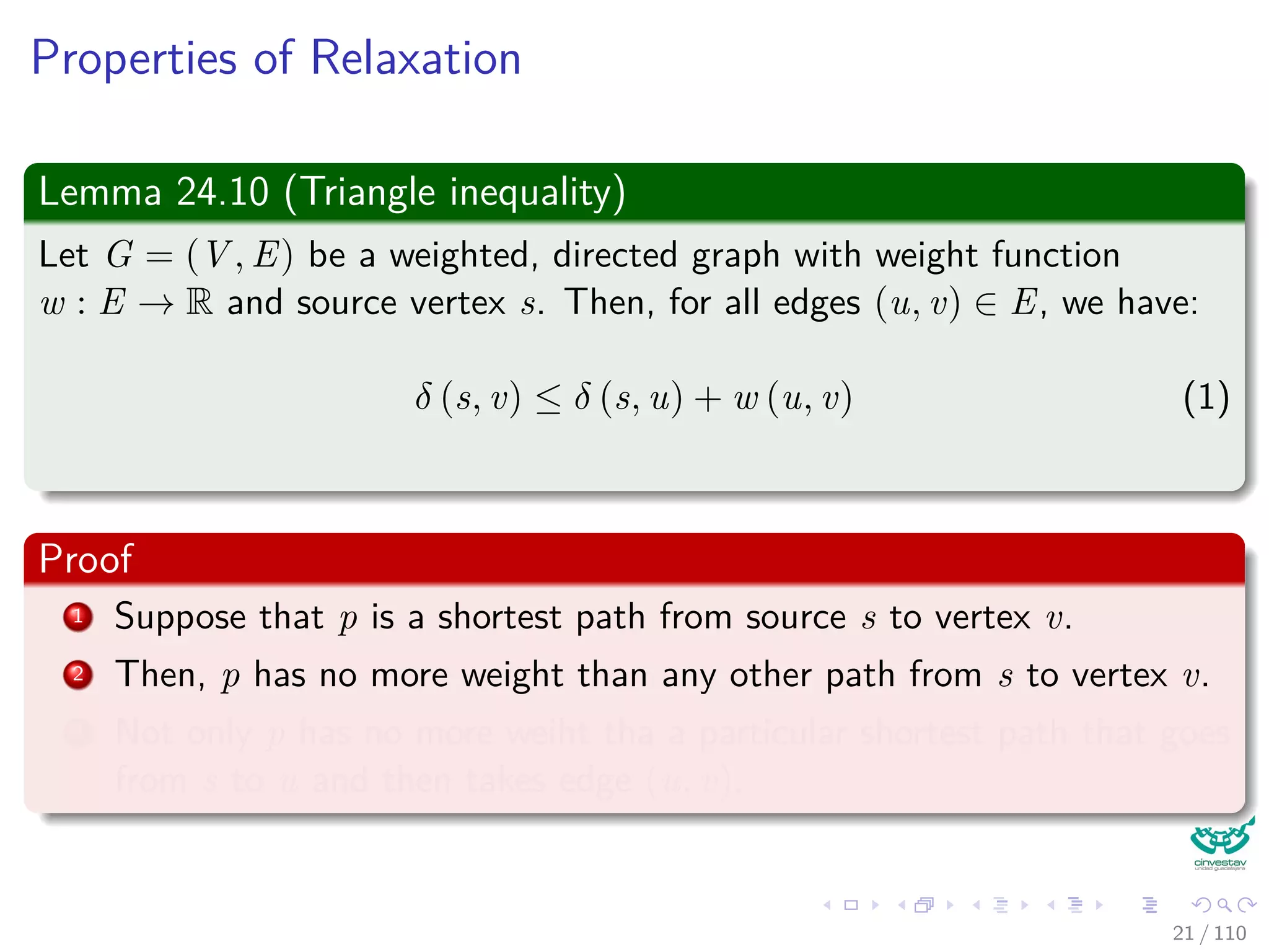
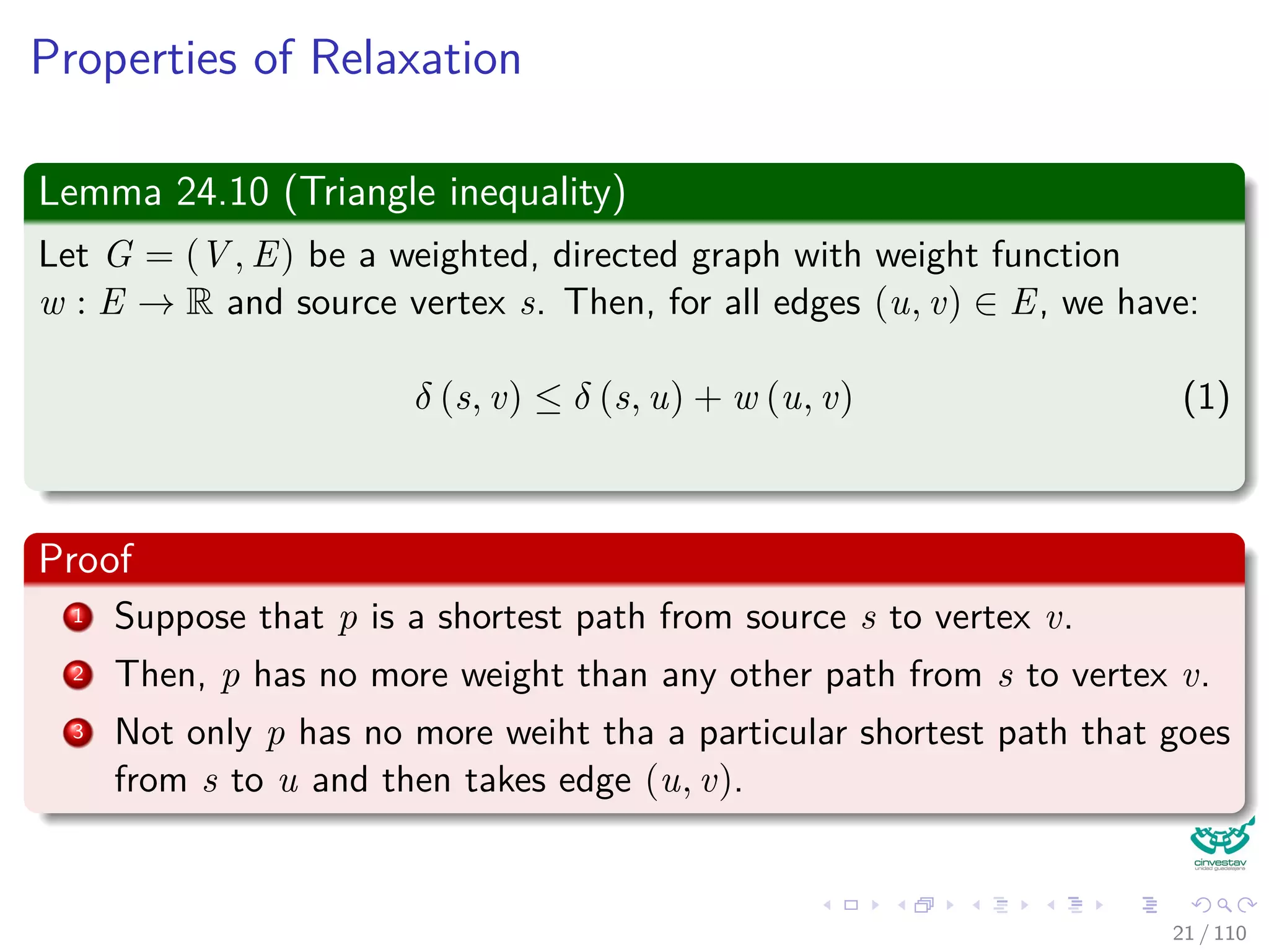

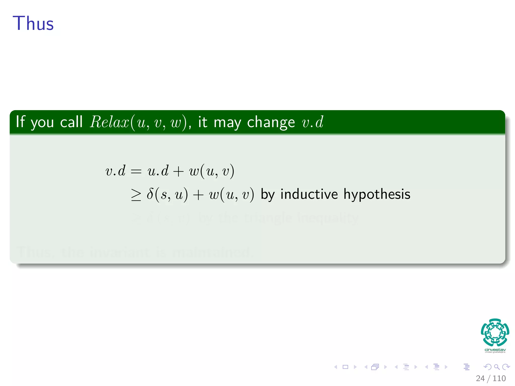
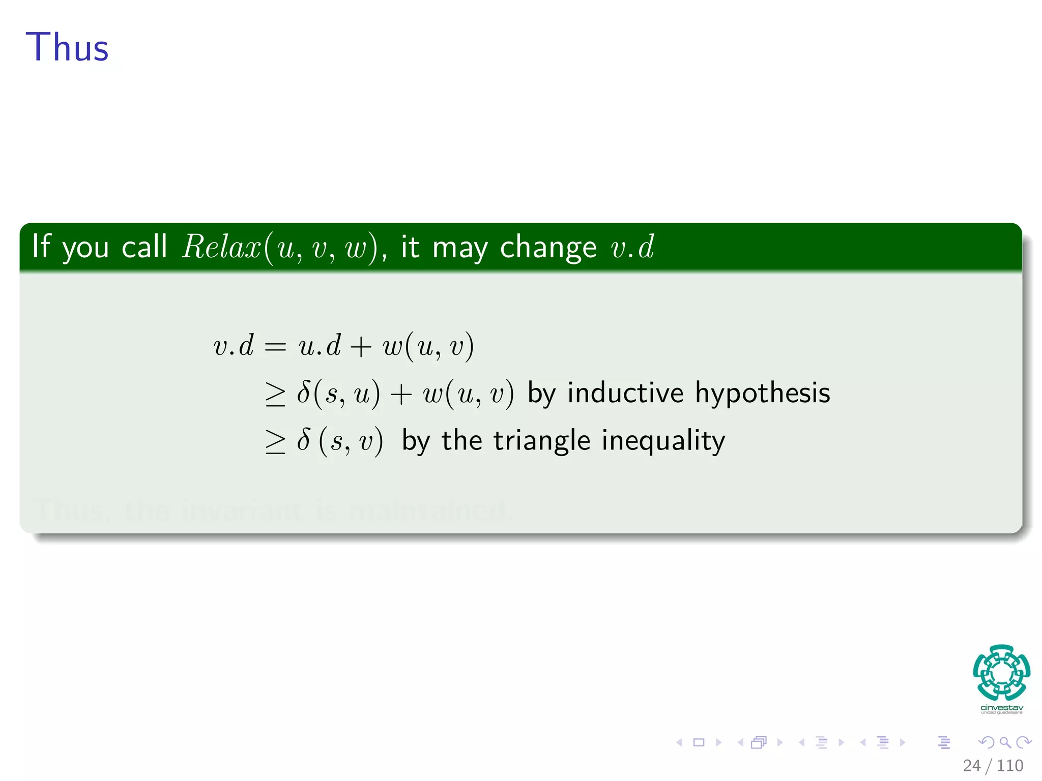
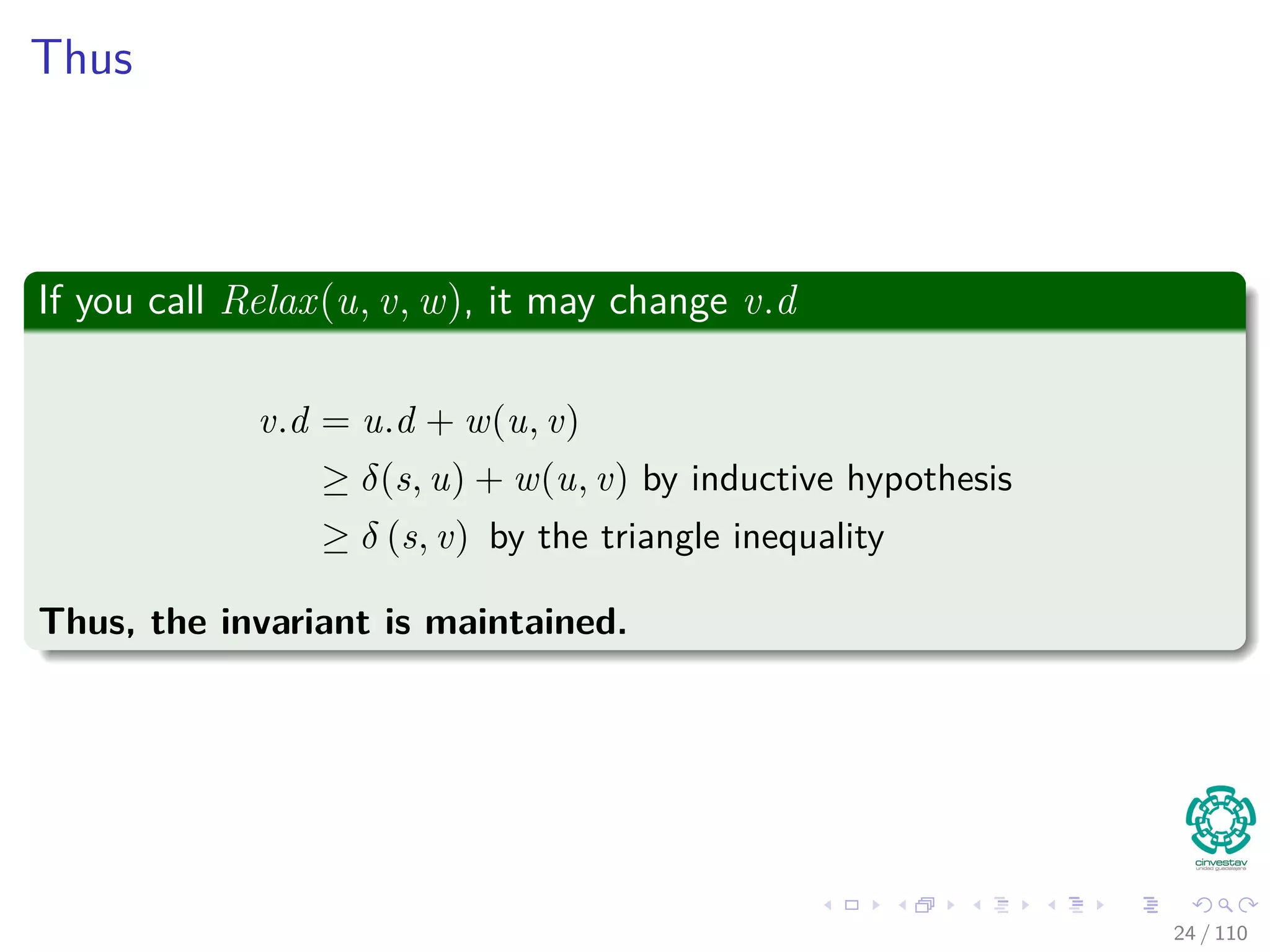
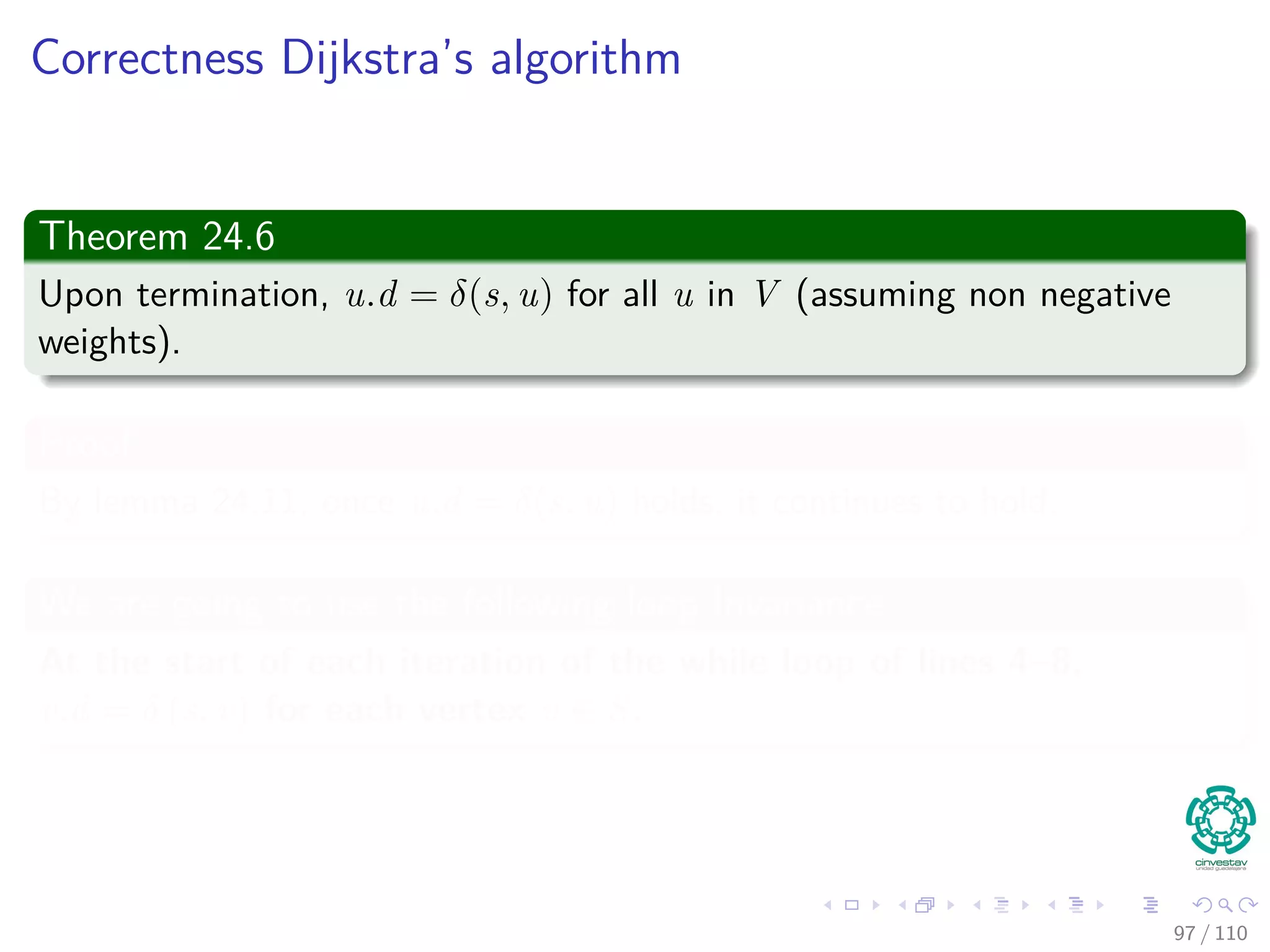
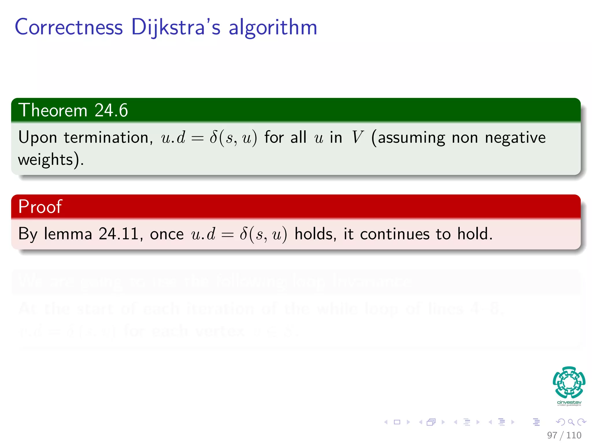
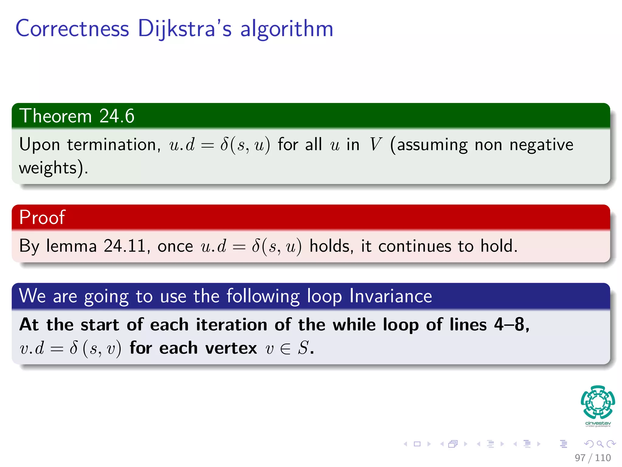
![Properties of Relaxation
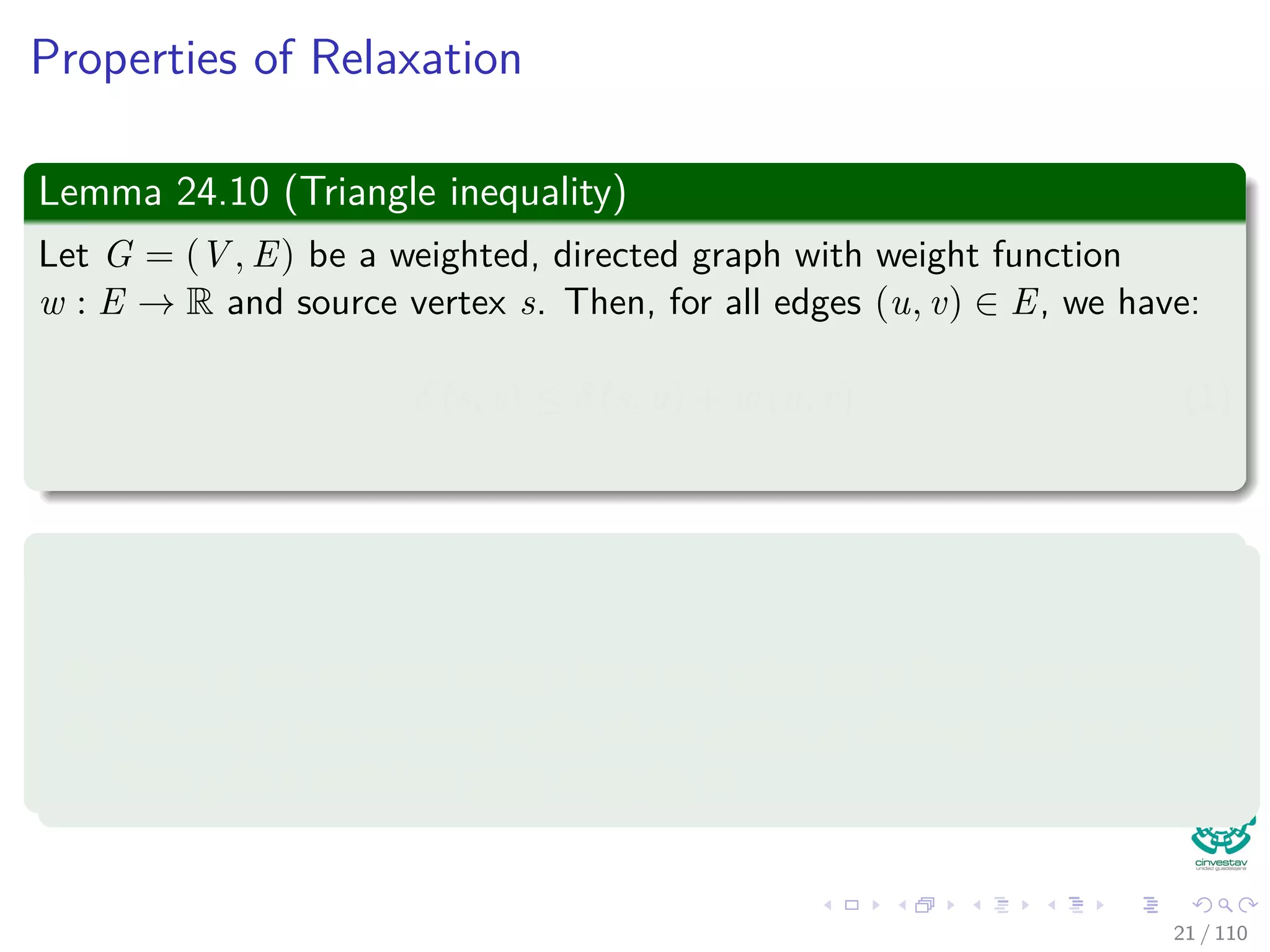
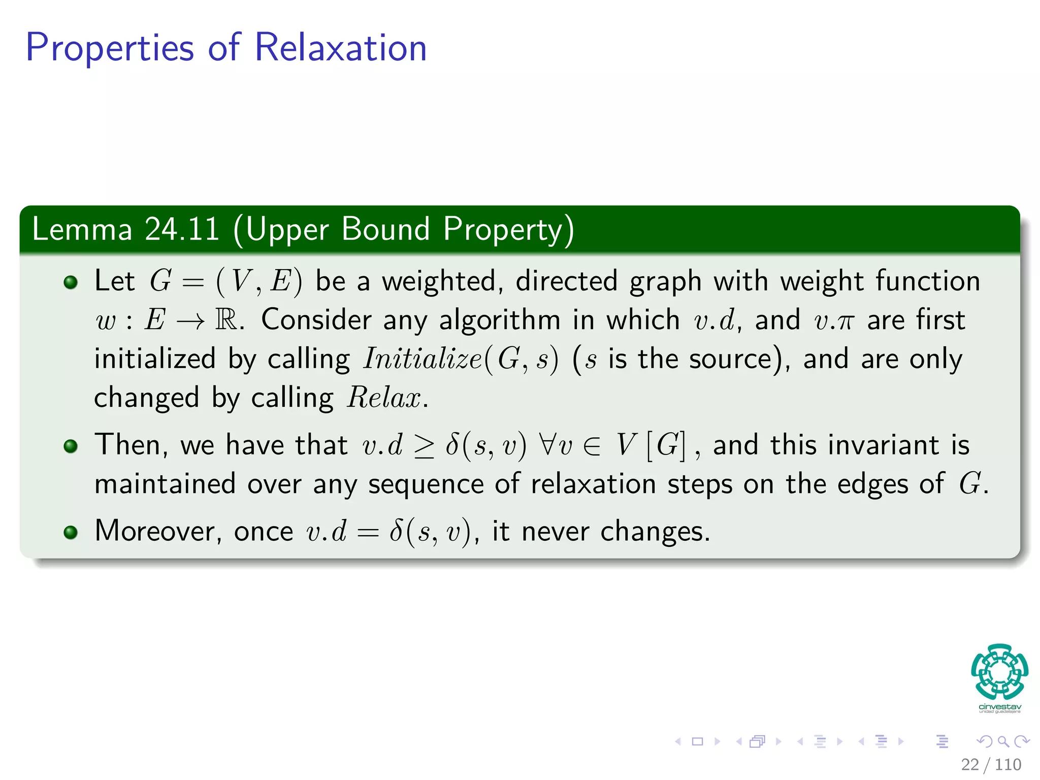
Lemma 24.11 (Upper Bound Property)
Let G = (V , E) be a weighted, directed graph with weight function
w : E → R. Consider any algorithm in which v.d, and v.π are first
initialized by calling Initialize(G, s) (s is the source), and are only
changed by calling Relax.
Then, we have that v.d ≥ δ(s, v) ∀v ∈ V [G] , and this invariant is
maintained over any sequence of relaxation steps on the edges of G.
Moreover, once v.d = δ(s, v), it never changes.
24 / 108](https://image.slidesharecdn.com/20single-sourceshorthestpath-151109143432-lva1-app6891/75/20-Single-Source-Shorthest-Path-59-2048.jpg)
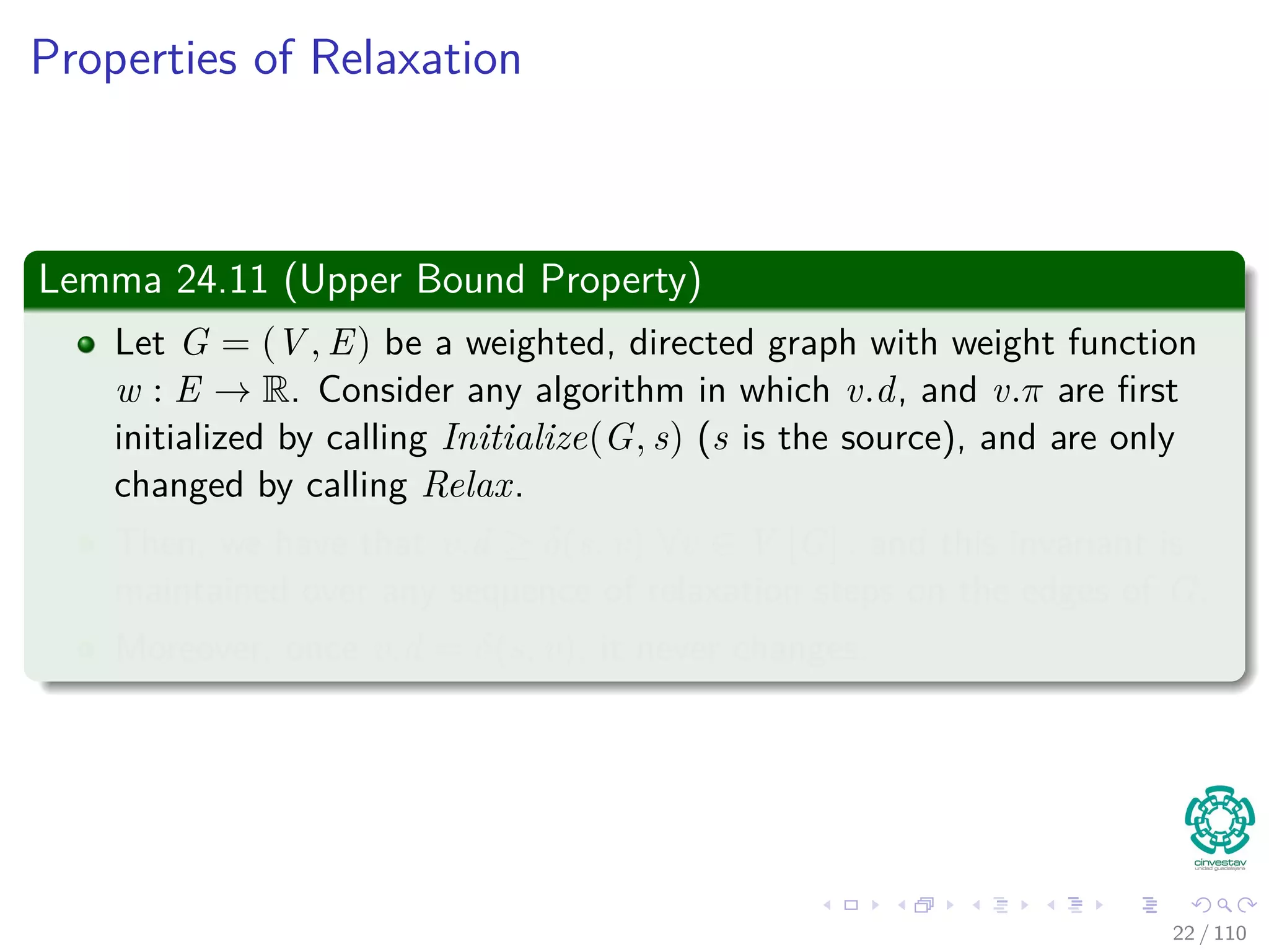
![Properties of Relaxation
Lemma 24.11 (Upper Bound Property)
Let G = (V , E) be a weighted, directed graph with weight function
w : E → R. Consider any algorithm in which v.d, and v.π are first
initialized by calling Initialize(G, s) (s is the source), and are only
changed by calling Relax.
Then, we have that v.d ≥ δ(s, v) ∀v ∈ V [G] , and this invariant is
maintained over any sequence of relaxation steps on the edges of G.
Moreover, once v.d = δ(s, v), it never changes.
24 / 108](https://image.slidesharecdn.com/20single-sourceshorthestpath-151109143432-lva1-app6891/75/20-Single-Source-Shorthest-Path-60-2048.jpg)
![Properties of Relaxation
Lemma 24.11 (Upper Bound Property)
Let G = (V , E) be a weighted, directed graph with weight function
w : E → R. Consider any algorithm in which v.d, and v.π are first
initialized by calling Initialize(G, s) (s is the source), and are only
changed by calling Relax.
Then, we have that v.d ≥ δ(s, v) ∀v ∈ V [G] , and this invariant is
maintained over any sequence of relaxation steps on the edges of G.
Moreover, once v.d = δ(s, v), it never changes.
24 / 108](https://image.slidesharecdn.com/20single-sourceshorthestpath-151109143432-lva1-app6891/75/20-Single-Source-Shorthest-Path-61-2048.jpg)


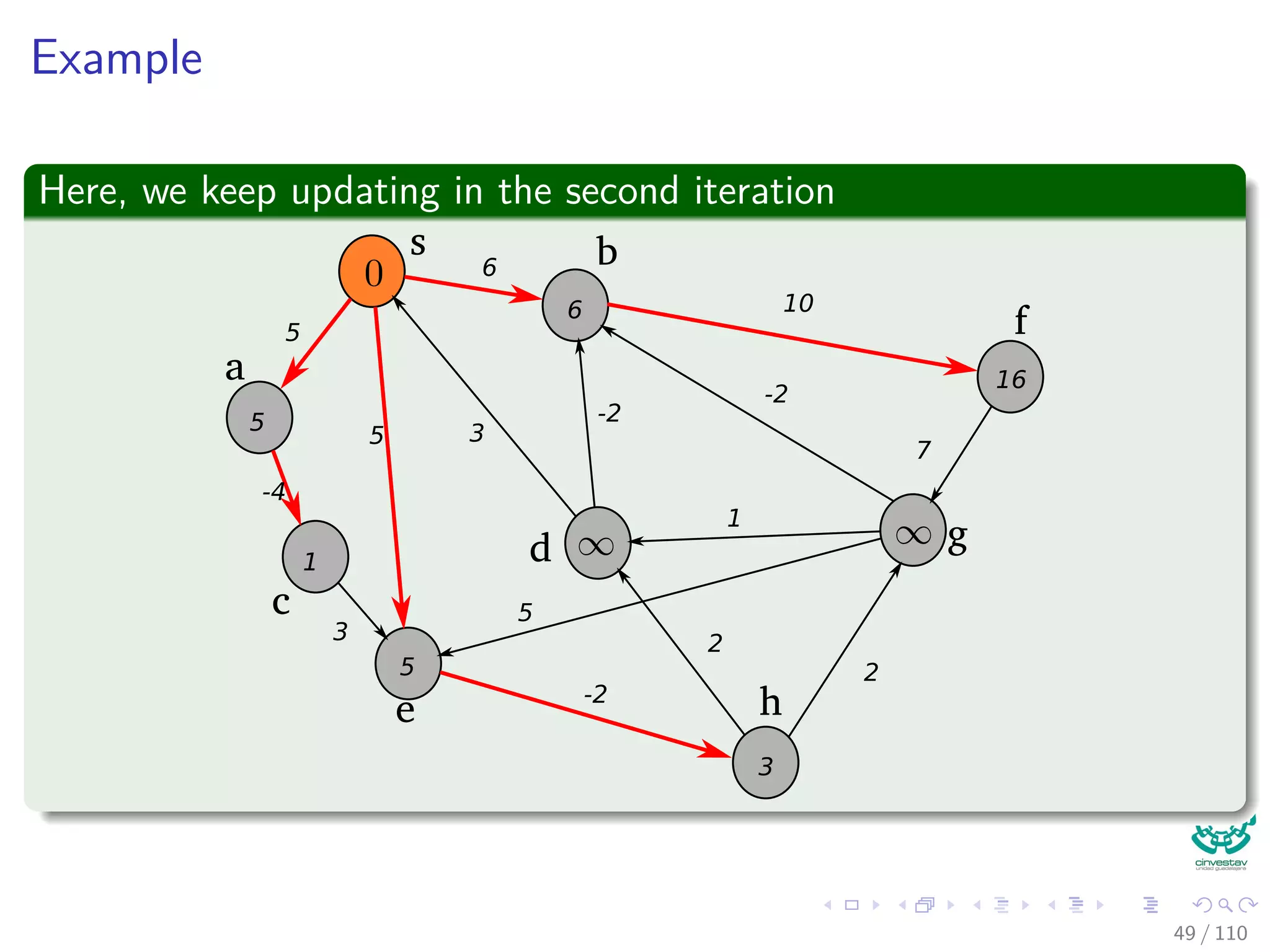
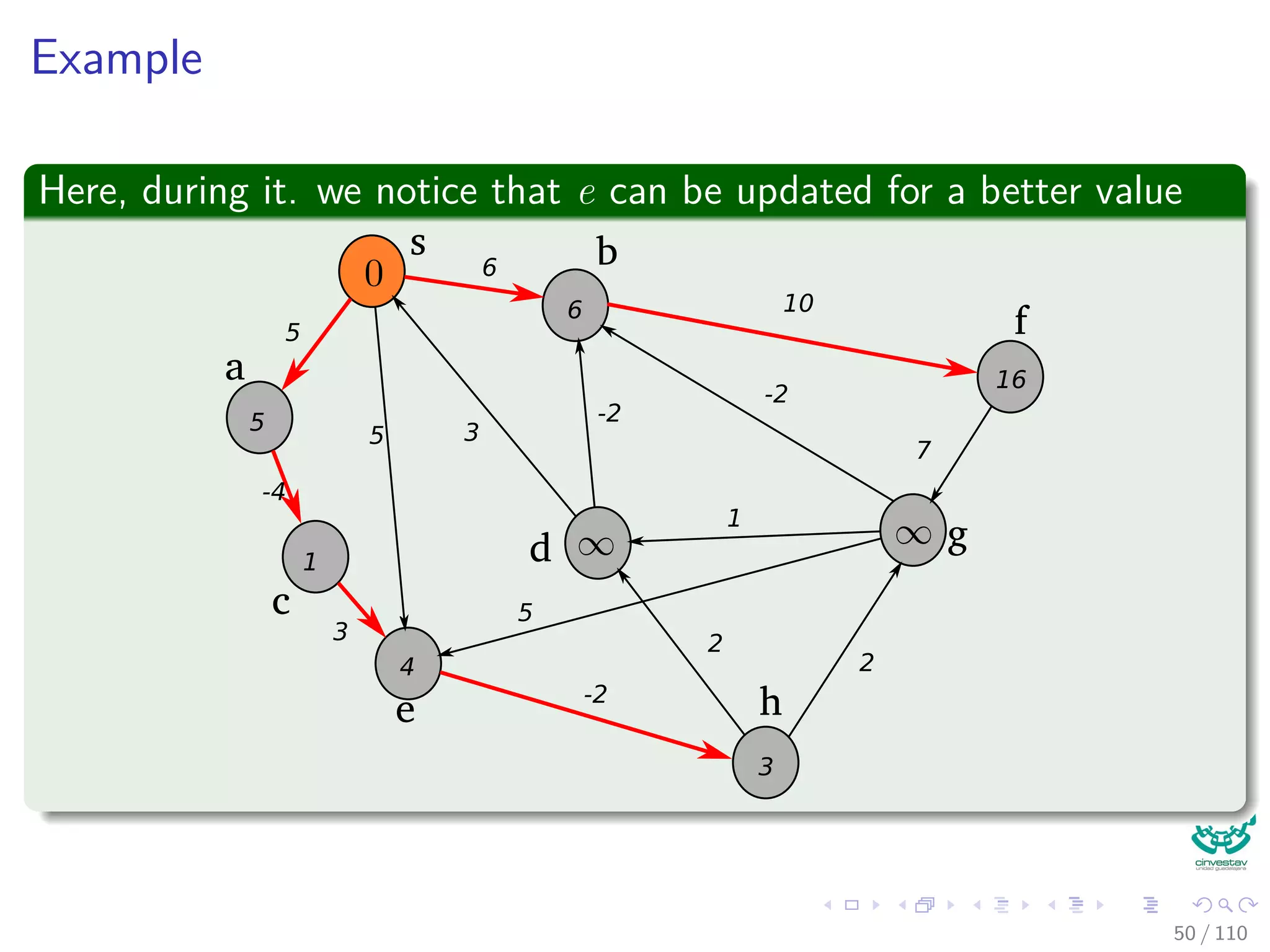
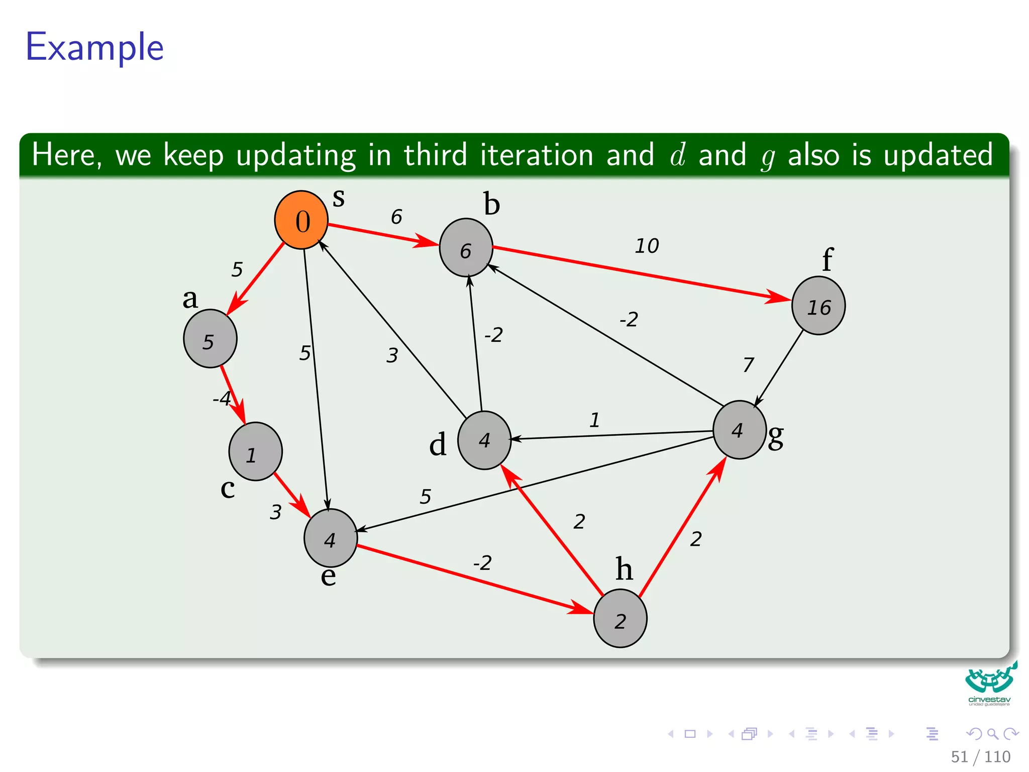
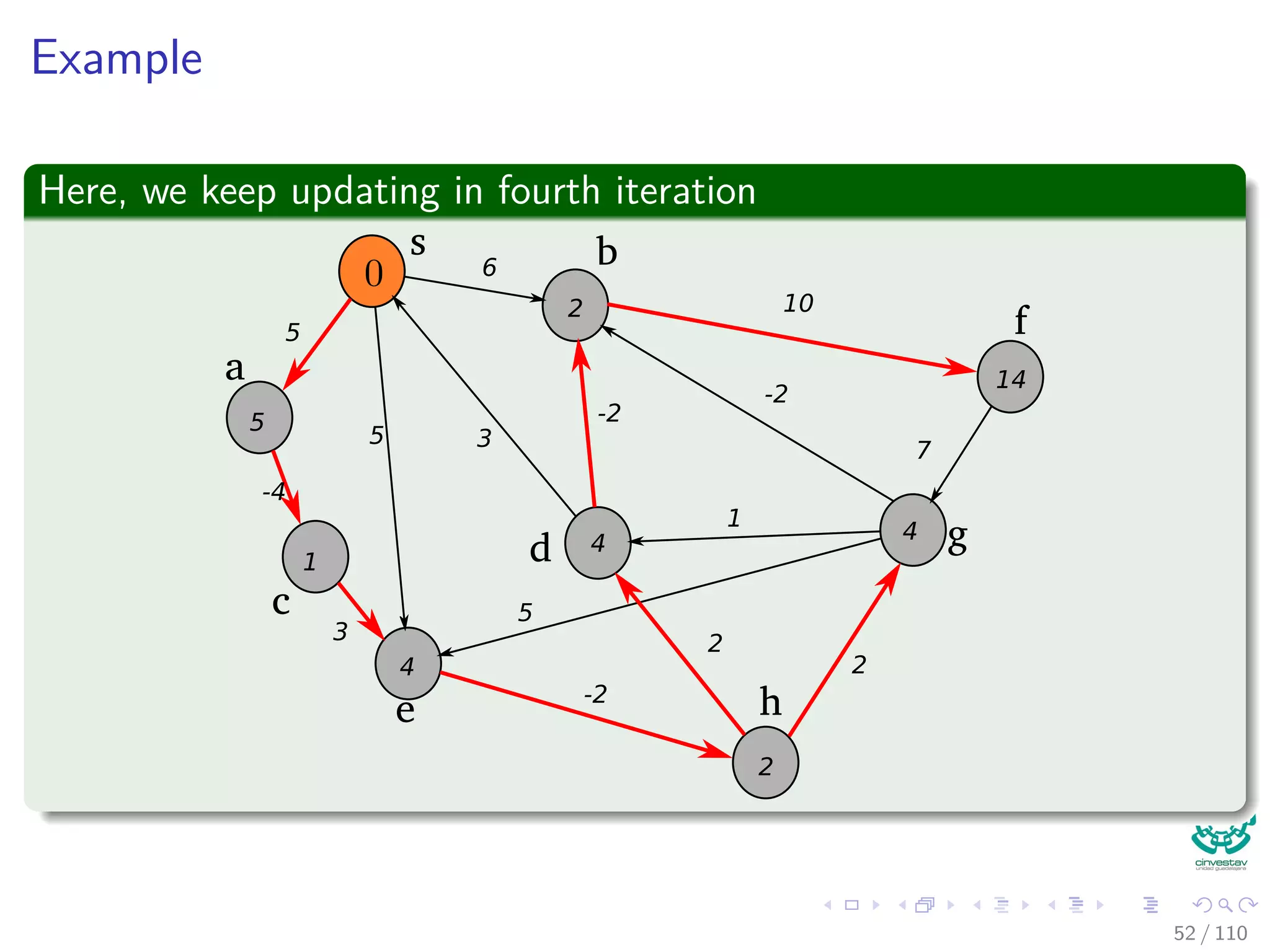
![Again the Bellman-Ford Algorithm
Bellman-Ford can have negative weight edges. It will “detect”
reachable negative weight cycles.
Bellman-Ford(G, s, w)
1 Initialize(G, s)
2 for i = 1 to |V [G]| − 1
3 for each (u, v) to E [G]
4 Relax(u, v, w) The Decision Part of the Dynamic
Programming for u.d and u.π.
5 for each (u, v) to E [G]
6 if v.d > u.d + w (u, v)
7 return false
8 return true
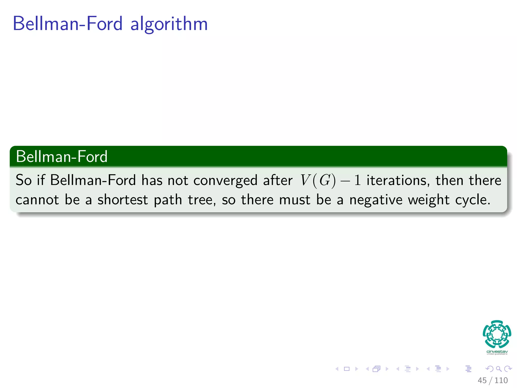
Observation
If Bellman-Ford has not converged after V (G) − 1 iterations, then
there cannot be a shortest path tree, so there must be a negative46 / 108](https://image.slidesharecdn.com/20single-sourceshorthestpath-151109143432-lva1-app6891/75/20-Single-Source-Shorthest-Path-127-2048.jpg)
![Again the Bellman-Ford Algorithm
Bellman-Ford can have negative weight edges. It will “detect”
reachable negative weight cycles.
Bellman-Ford(G, s, w)
1 Initialize(G, s)
2 for i = 1 to |V [G]| − 1
3 for each (u, v) to E [G]
4 Relax(u, v, w) The Decision Part of the Dynamic
Programming for u.d and u.π.
5 for each (u, v) to E [G]
6 if v.d > u.d + w (u, v)
7 return false
8 return true
Observation
If Bellman-Ford has not converged after V (G) − 1 iterations, then
there cannot be a shortest path tree, so there must be a negative46 / 108](https://image.slidesharecdn.com/20single-sourceshorthestpath-151109143432-lva1-app6891/75/20-Single-Source-Shorthest-Path-128-2048.jpg)


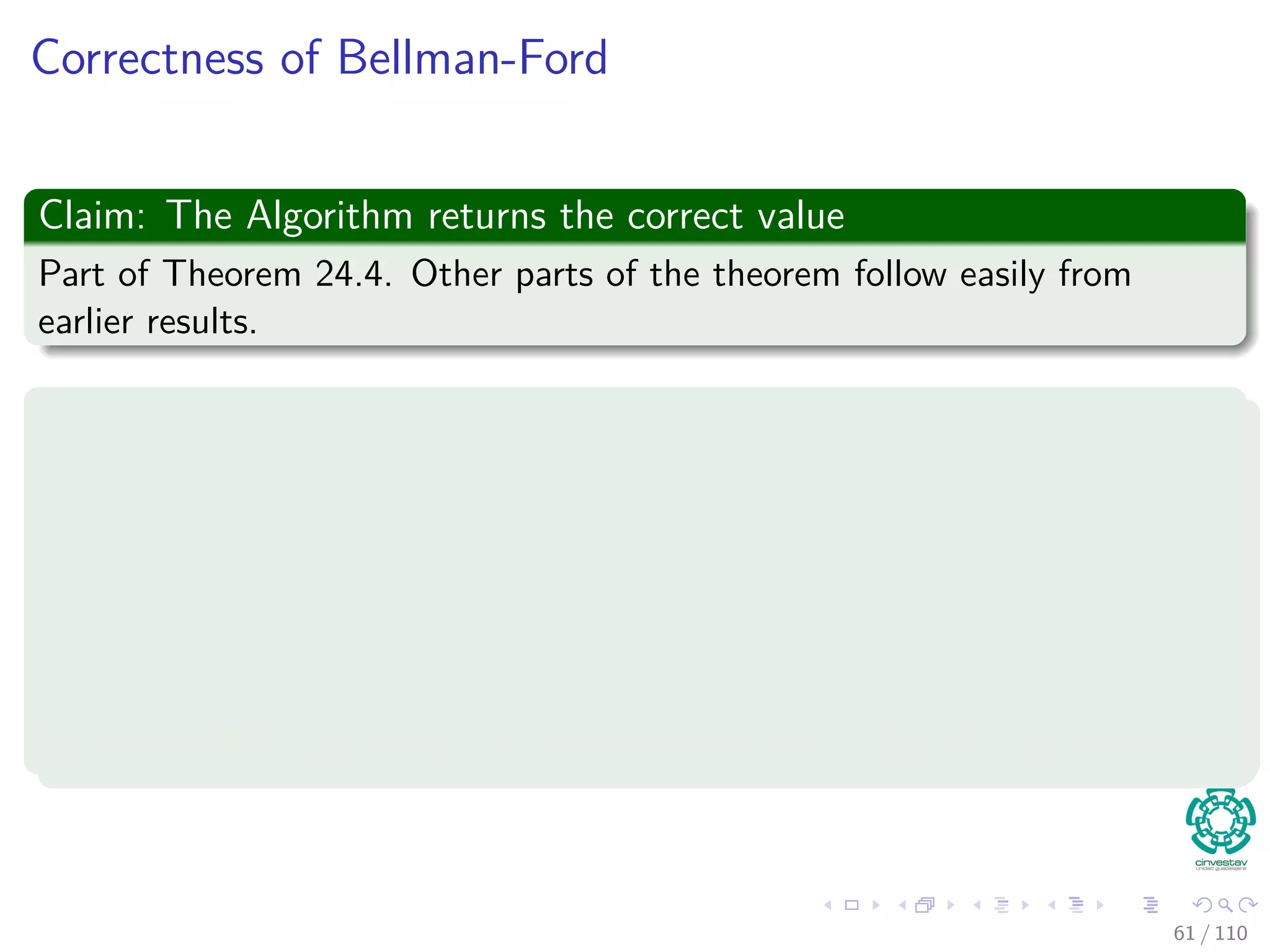

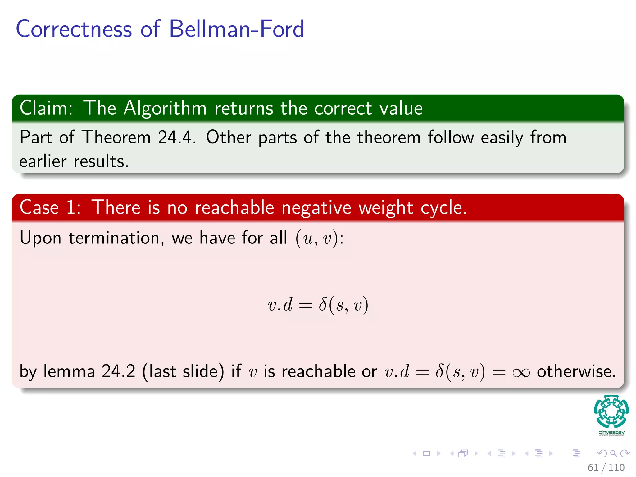
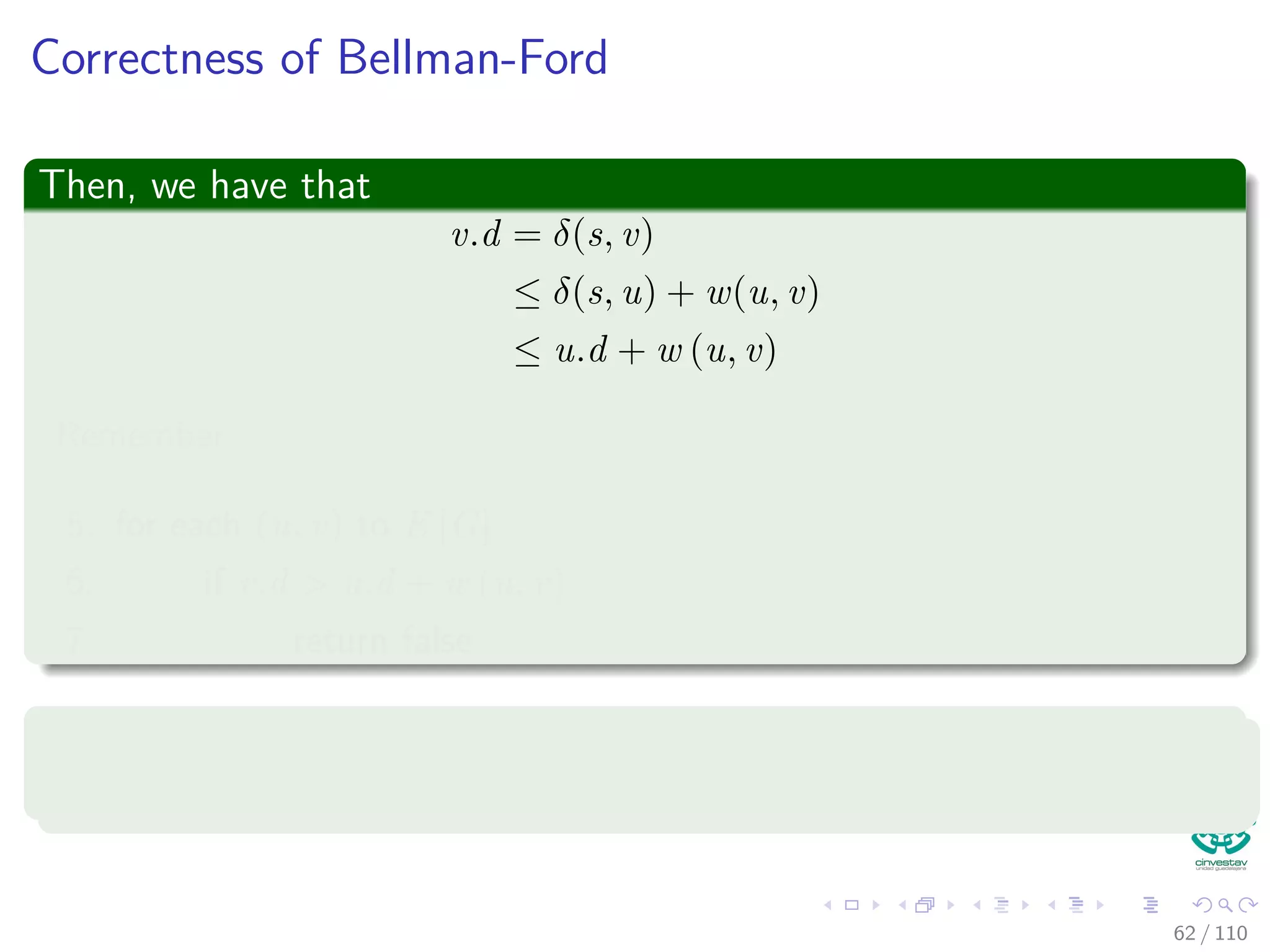
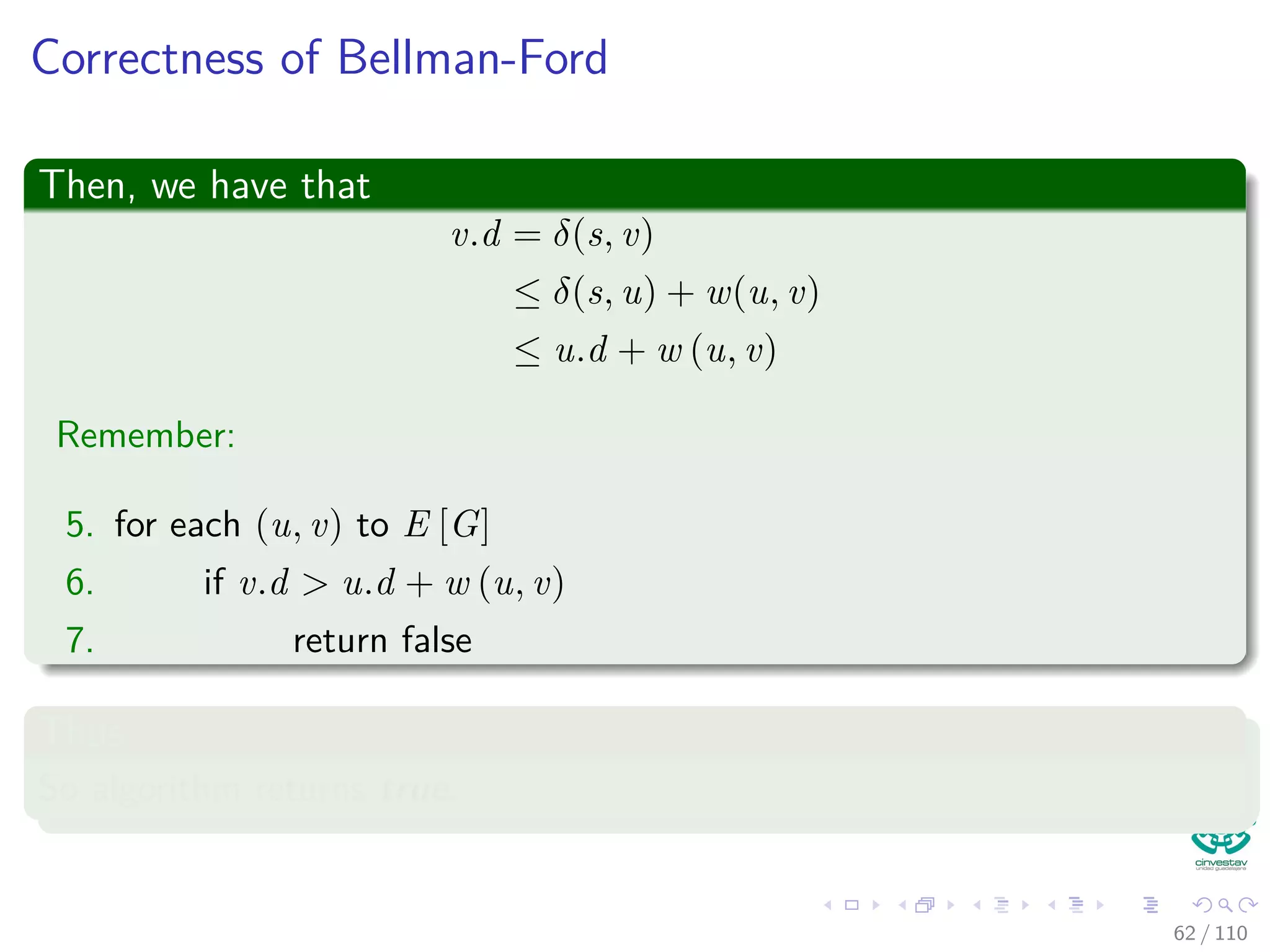
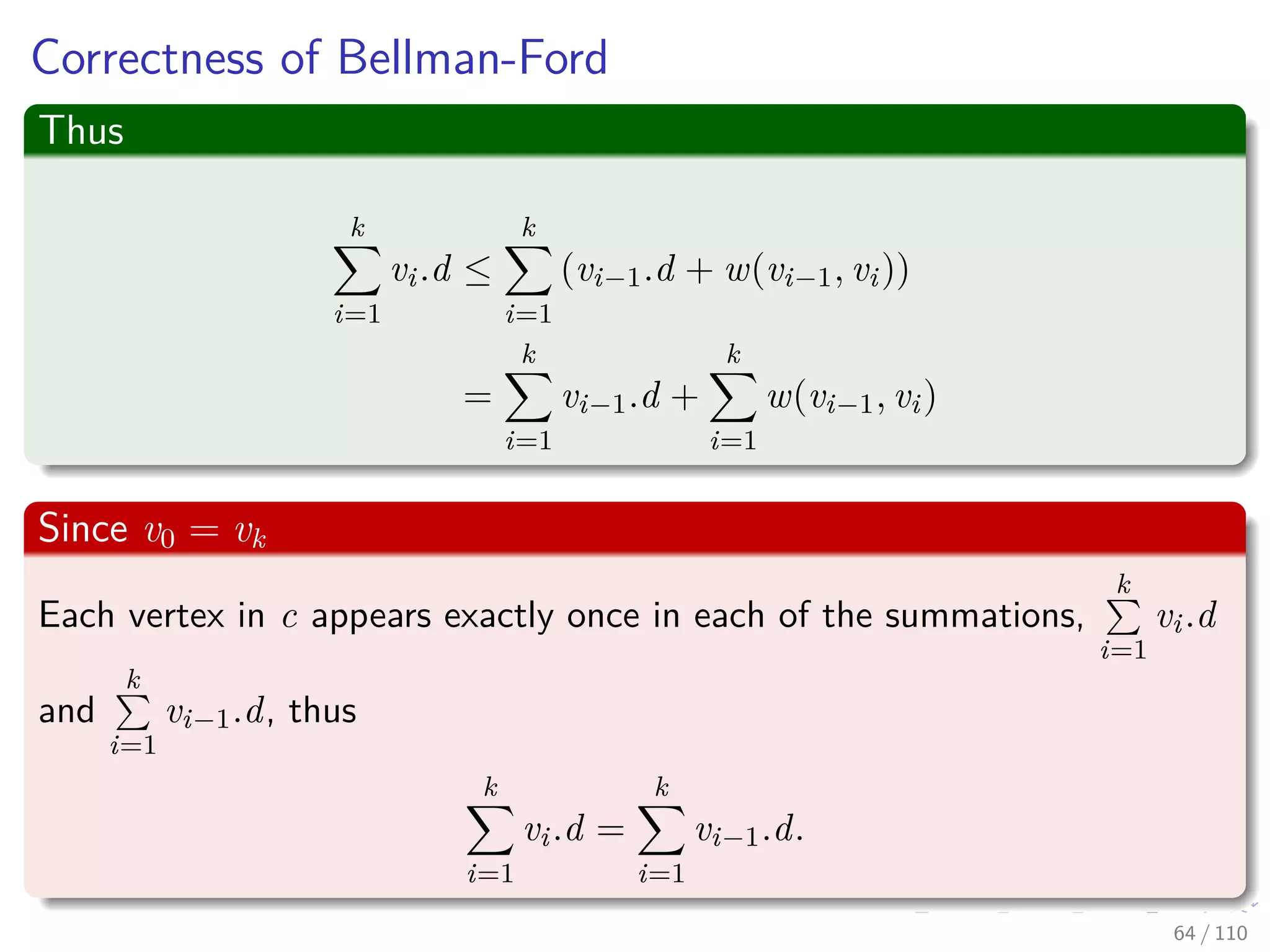
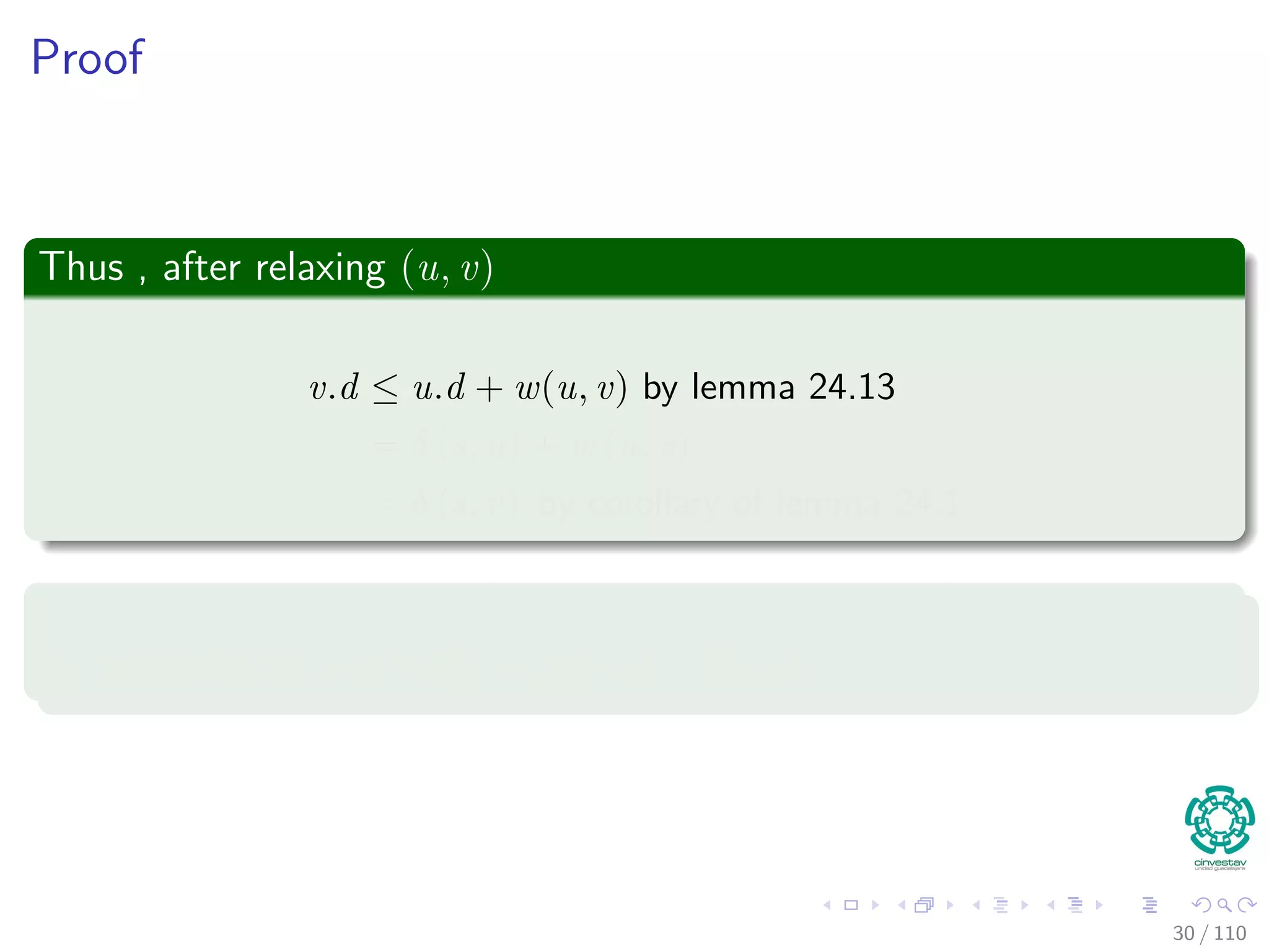
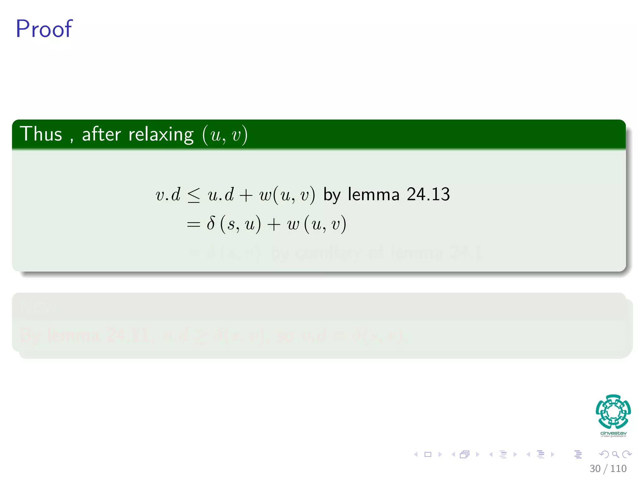
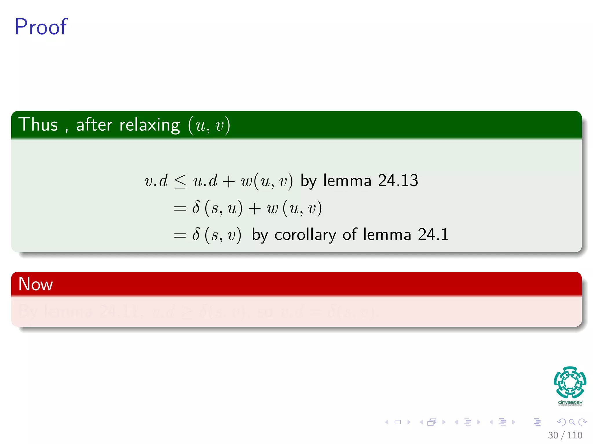
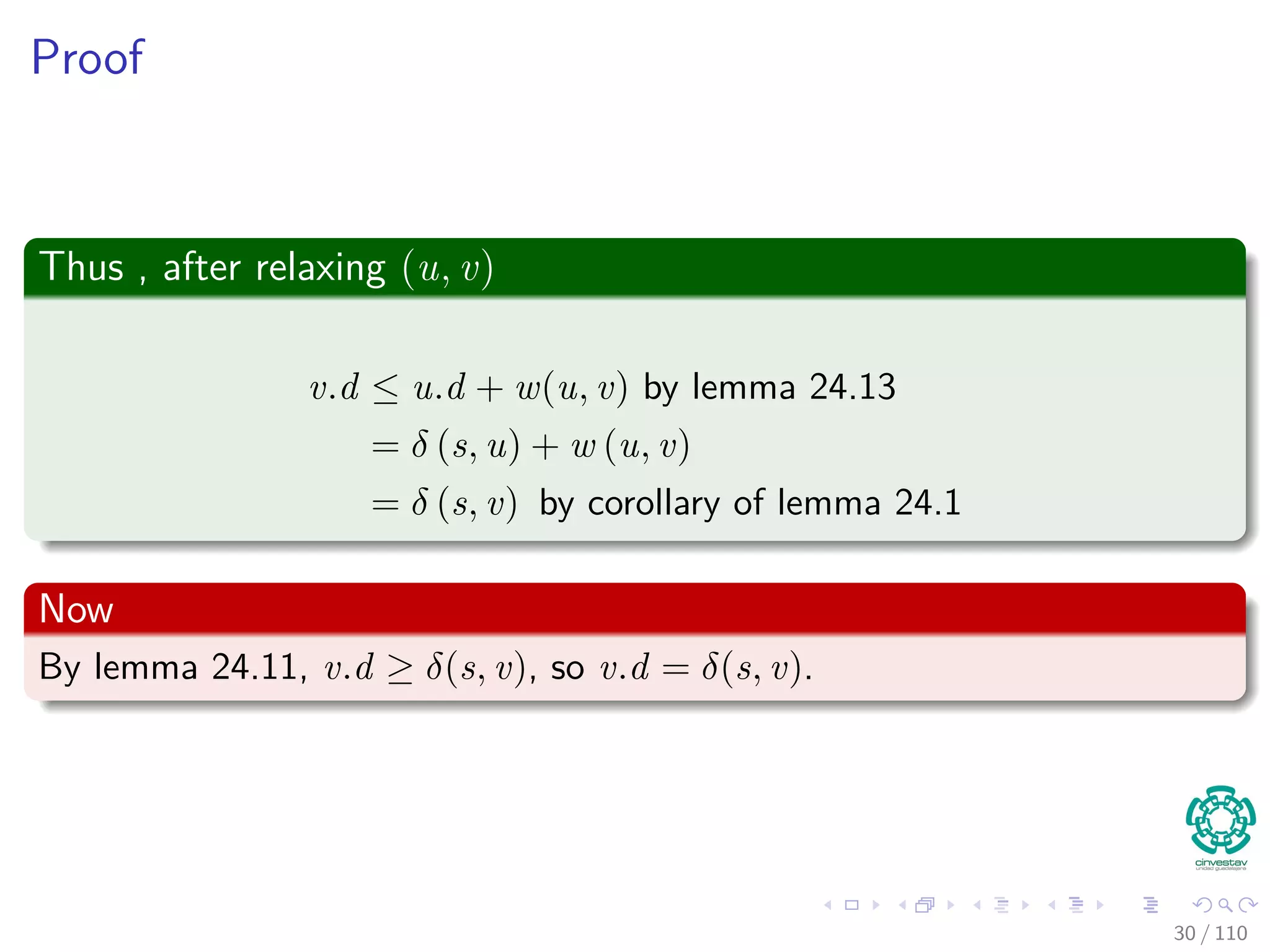
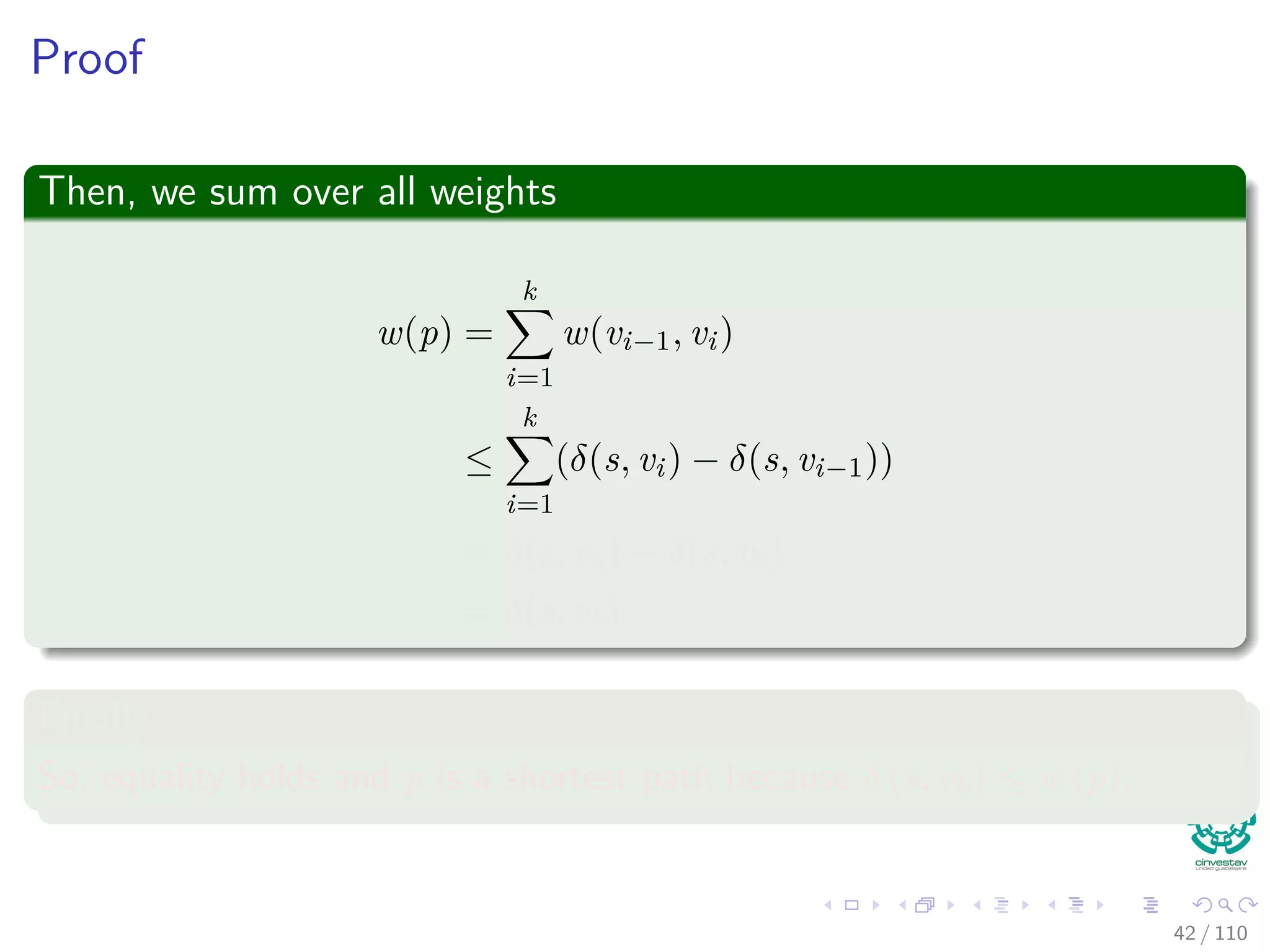
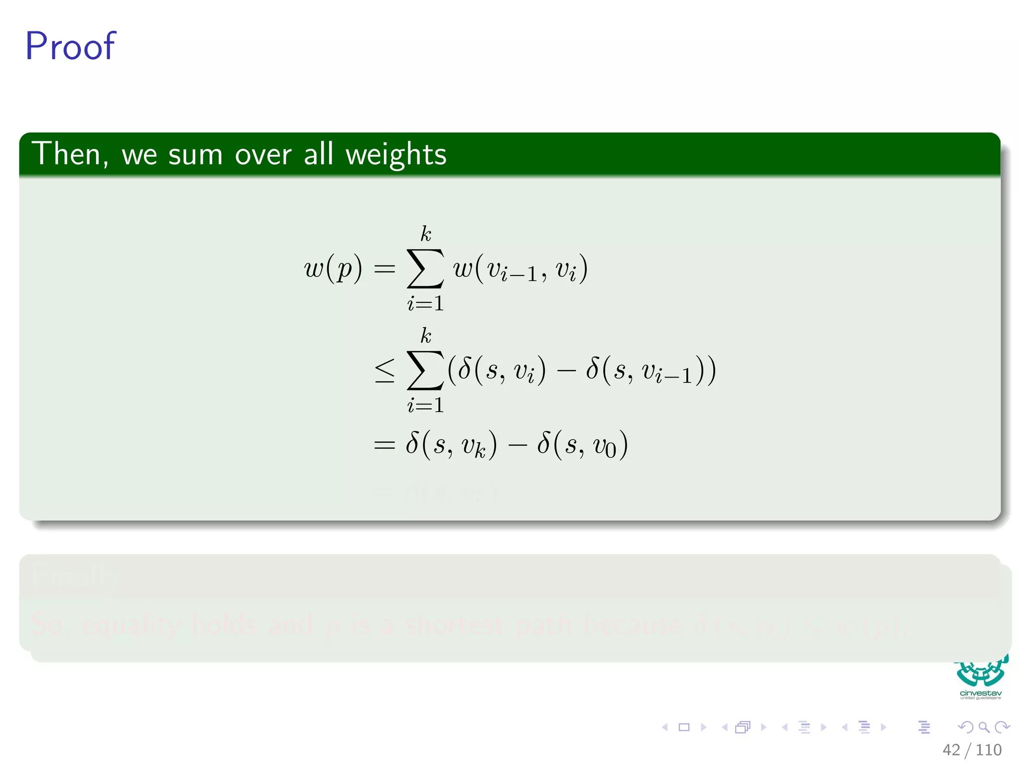
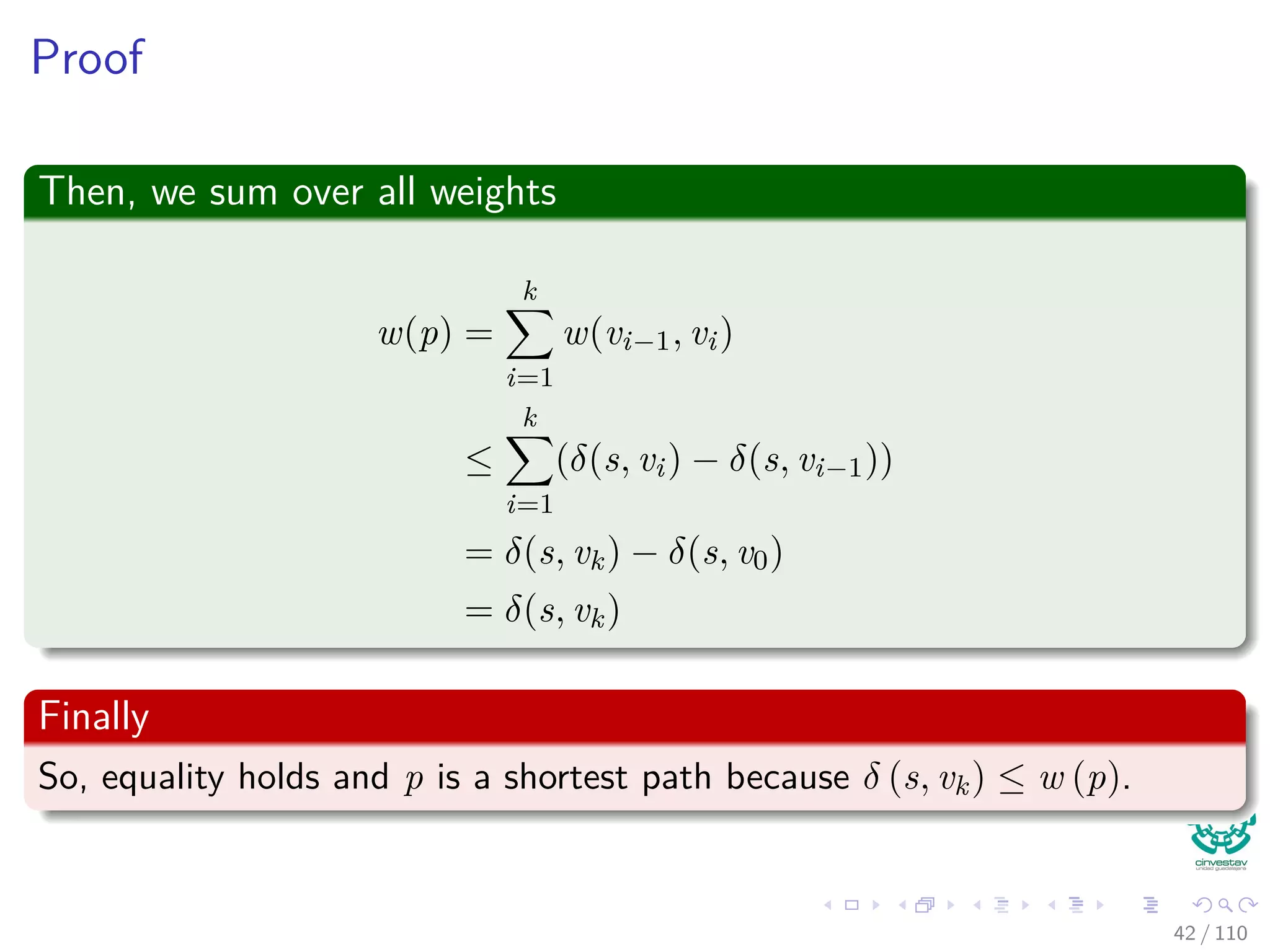
![Correctness of Bellman-Ford
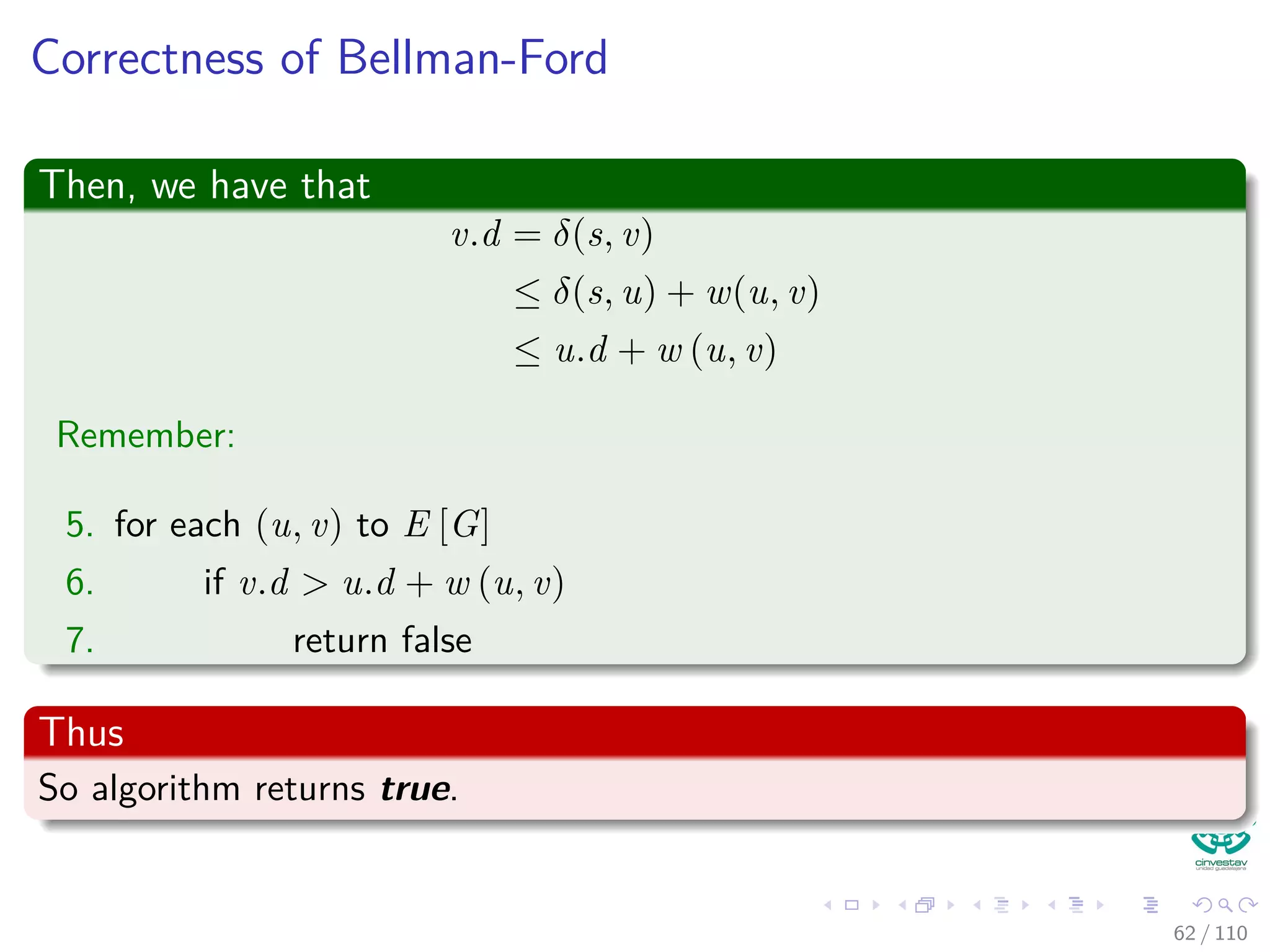
Then, we have that
v.d = δ(s, v)
≤ δ(s, u) + w(u, v)
≤ u.d + w (u, v)
Remember:
5. for each (u, v) to E [G]
6. if v.d > u.d + w (u, v)
7. return false
Thus
So algorithm returns true.
60 / 108](https://image.slidesharecdn.com/20single-sourceshorthestpath-151109143432-lva1-app6891/75/20-Single-Source-Shorthest-Path-150-2048.jpg)
![Correctness of Bellman-Ford
Then, we have that
v.d = δ(s, v)
≤ δ(s, u) + w(u, v)
≤ u.d + w (u, v)
Remember:
5. for each (u, v) to E [G]
6. if v.d > u.d + w (u, v)
7. return false
Thus
So algorithm returns true.
60 / 108](https://image.slidesharecdn.com/20single-sourceshorthestpath-151109143432-lva1-app6891/75/20-Single-Source-Shorthest-Path-151-2048.jpg)
![Correctness of Bellman-Ford
Then, we have that
v.d = δ(s, v)
≤ δ(s, u) + w(u, v)
≤ u.d + w (u, v)
Remember:
5. for each (u, v) to E [G]
6. if v.d > u.d + w (u, v)
7. return false
Thus
So algorithm returns true.
60 / 108](https://image.slidesharecdn.com/20single-sourceshorthestpath-151109143432-lva1-app6891/75/20-Single-Source-Shorthest-Path-152-2048.jpg)
![Correctness of Bellman-Ford
Then, we have that
v.d = δ(s, v)
≤ δ(s, u) + w(u, v)
≤ u.d + w (u, v)
Remember:
5. for each (u, v) to E [G]
6. if v.d > u.d + w (u, v)
7. return false
Thus
So algorithm returns true.
60 / 108](https://image.slidesharecdn.com/20single-sourceshorthestpath-151109143432-lva1-app6891/75/20-Single-Source-Shorthest-Path-153-2048.jpg)
![Correctness of Bellman-Ford
Then, we have that
v.d = δ(s, v)
≤ δ(s, u) + w(u, v)
≤ u.d + w (u, v)
Remember:
5. for each (u, v) to E [G]
6. if v.d > u.d + w (u, v)
7. return false
Thus
So algorithm returns true.
60 / 108](https://image.slidesharecdn.com/20single-sourceshorthestpath-151109143432-lva1-app6891/75/20-Single-Source-Shorthest-Path-154-2048.jpg)
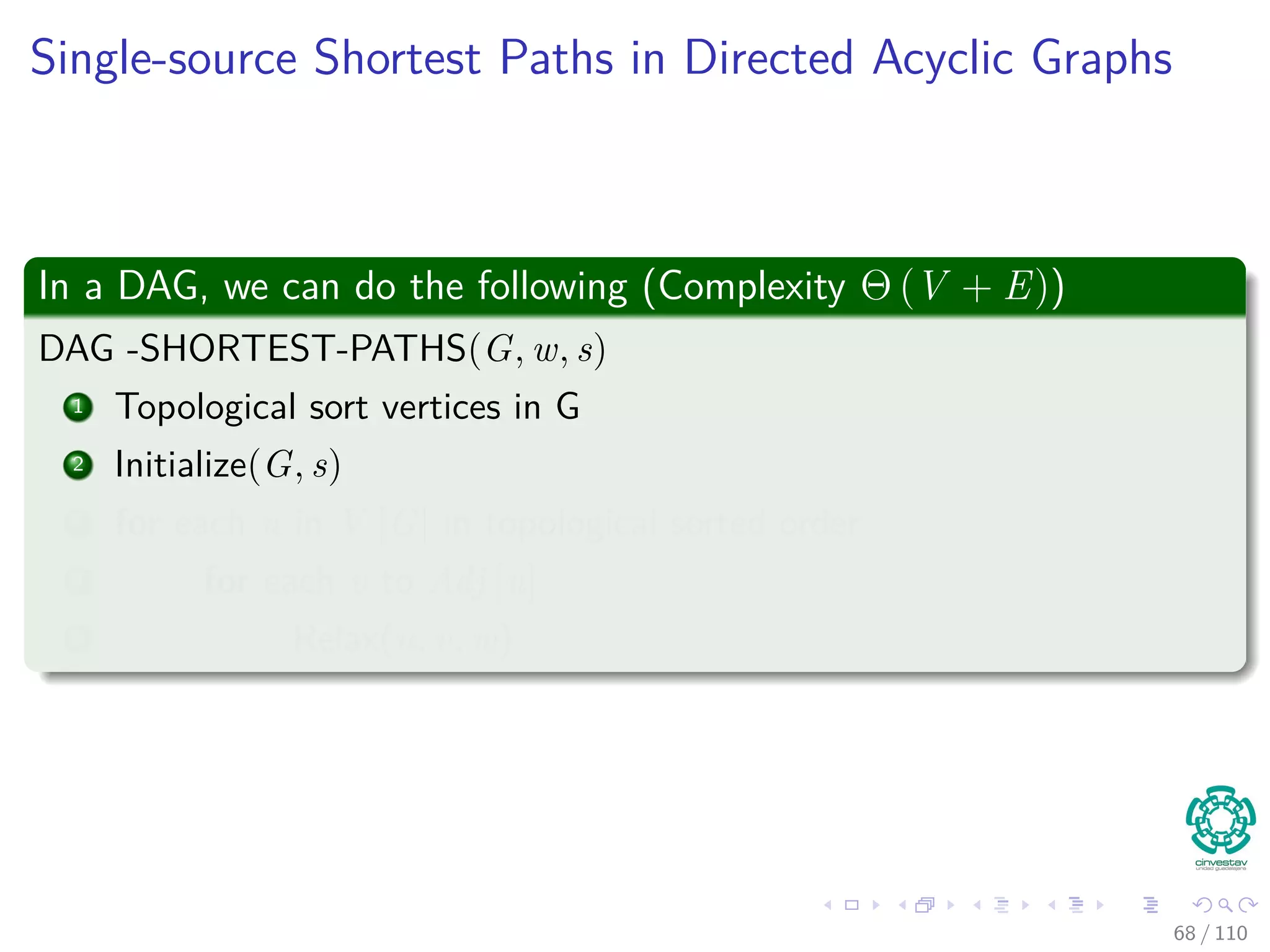

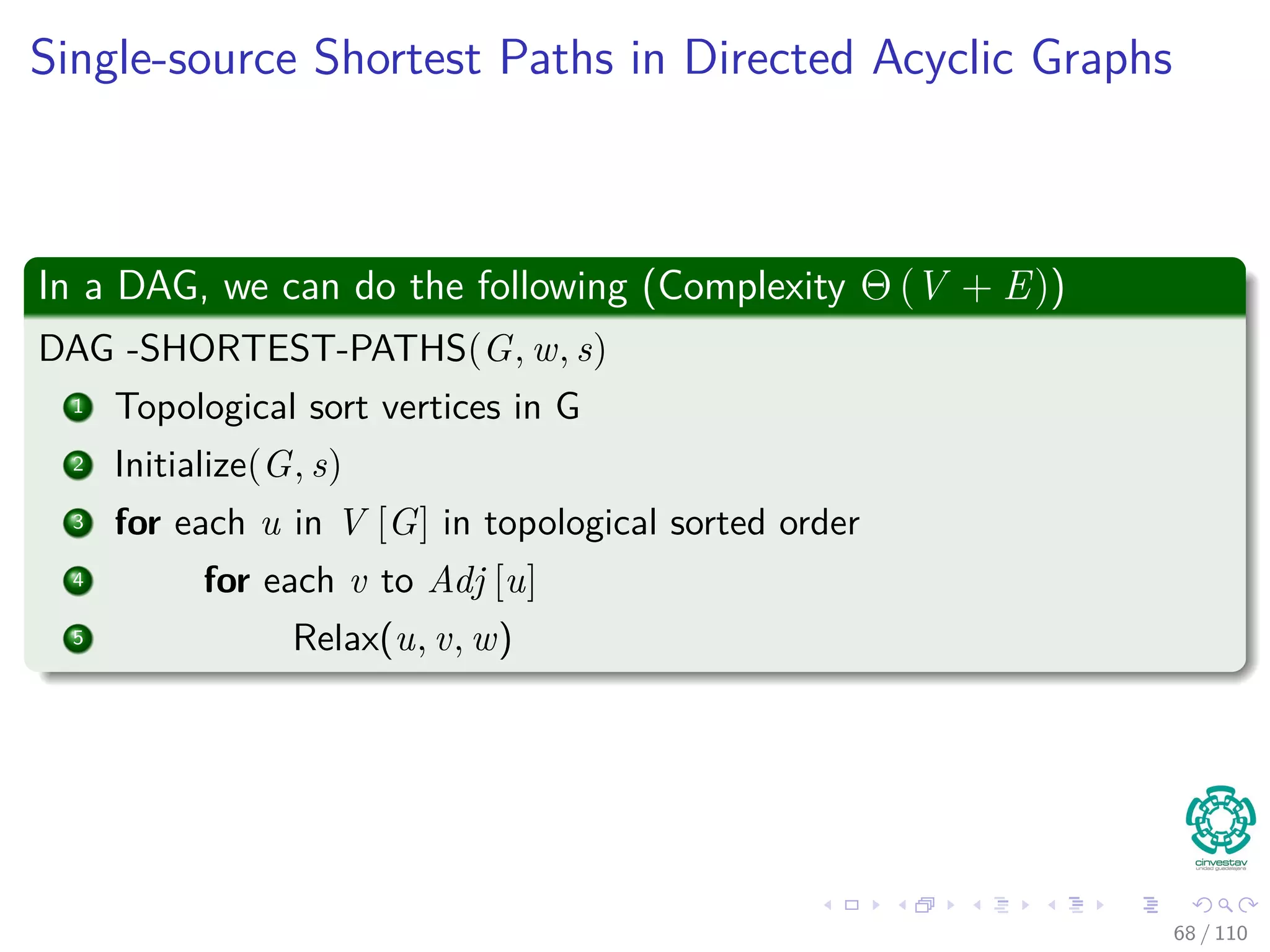

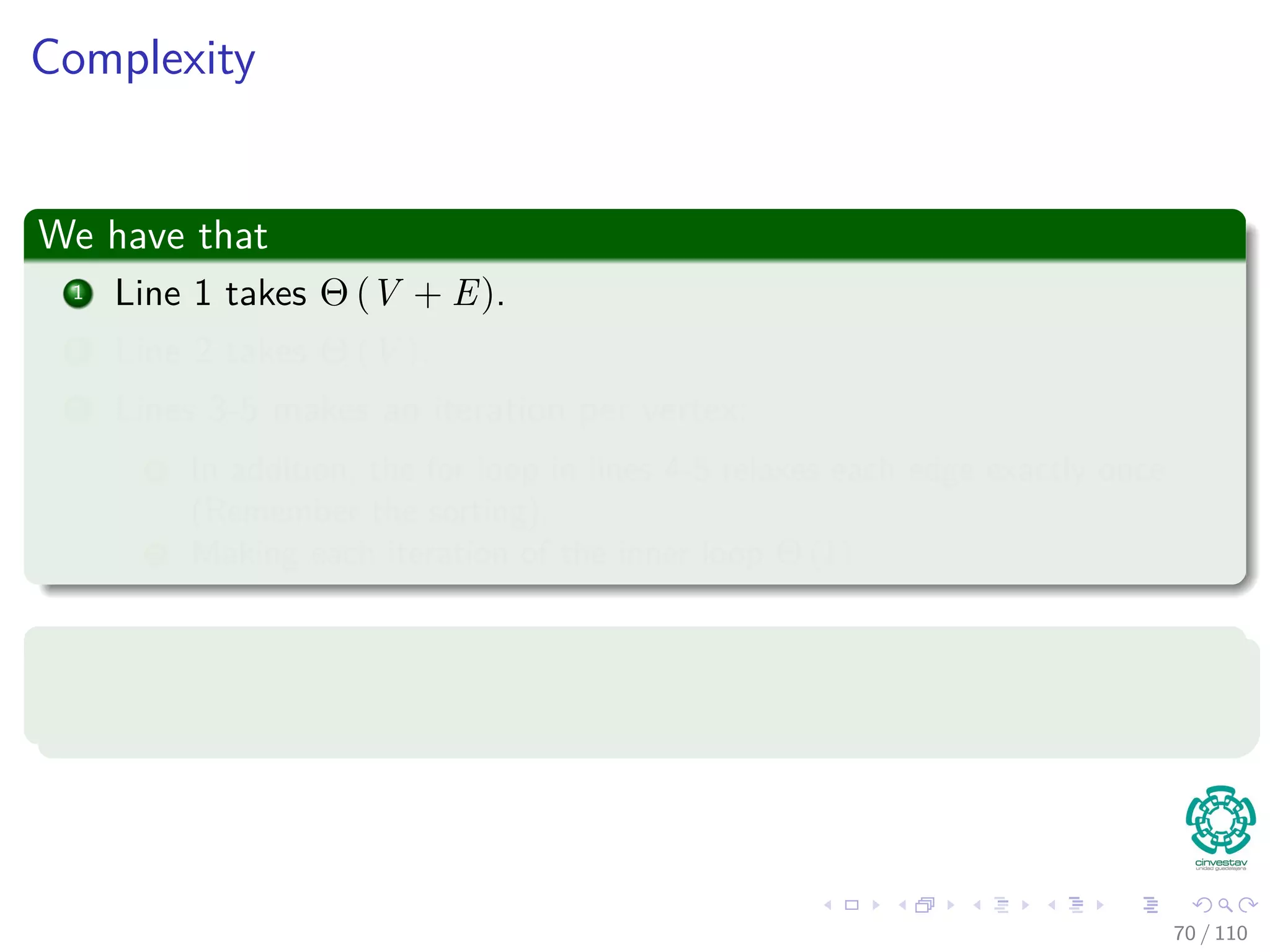

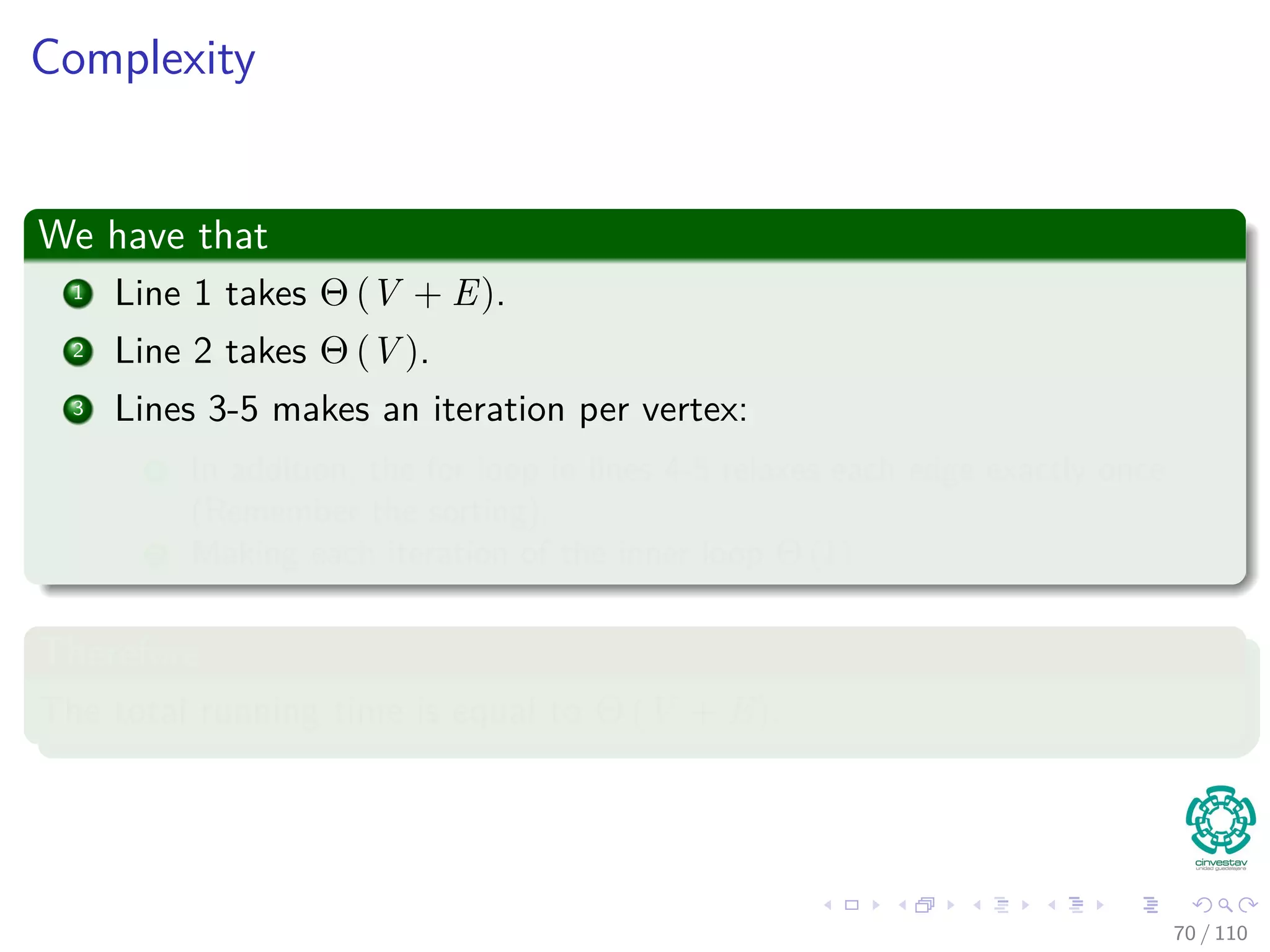
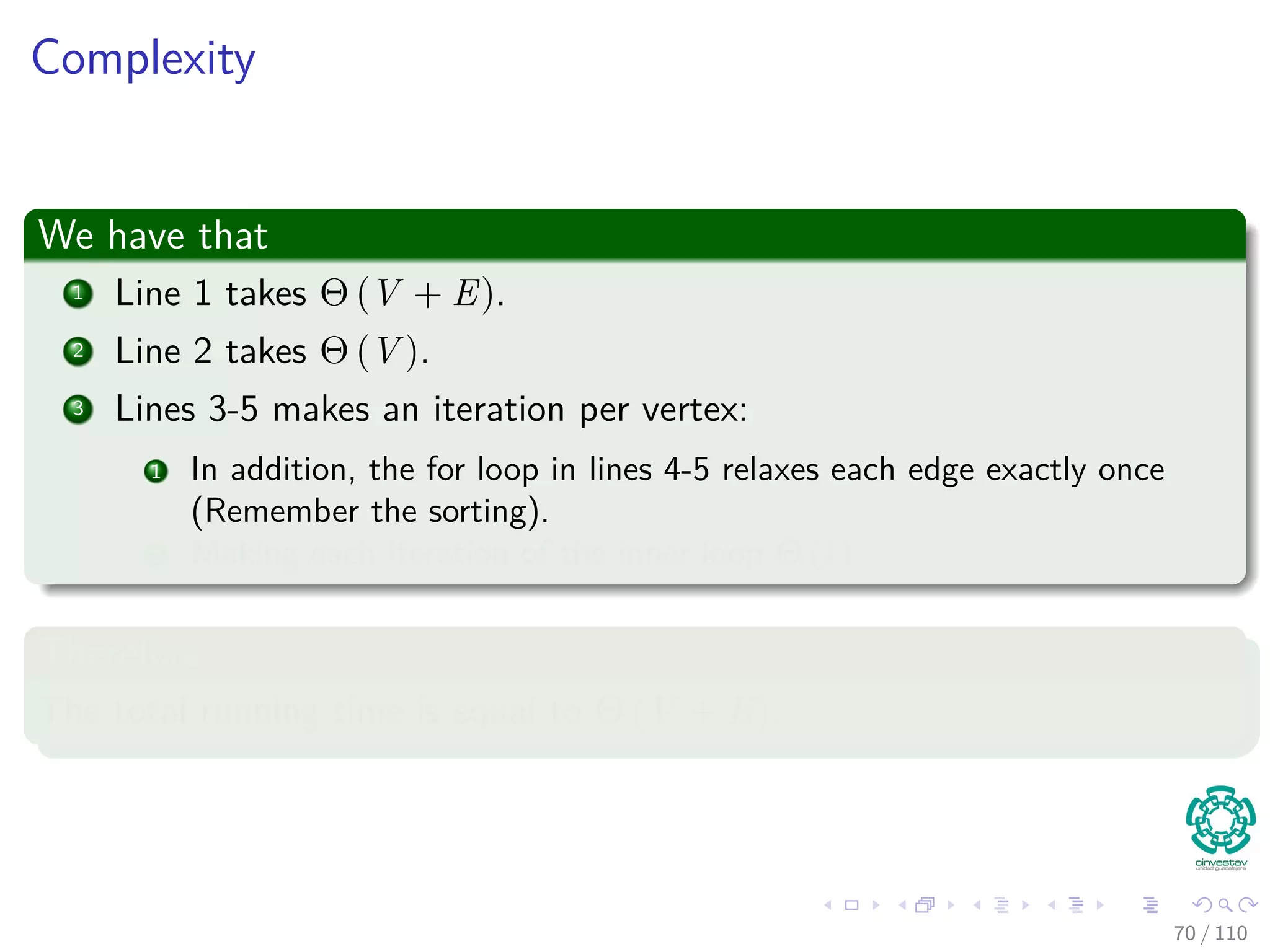
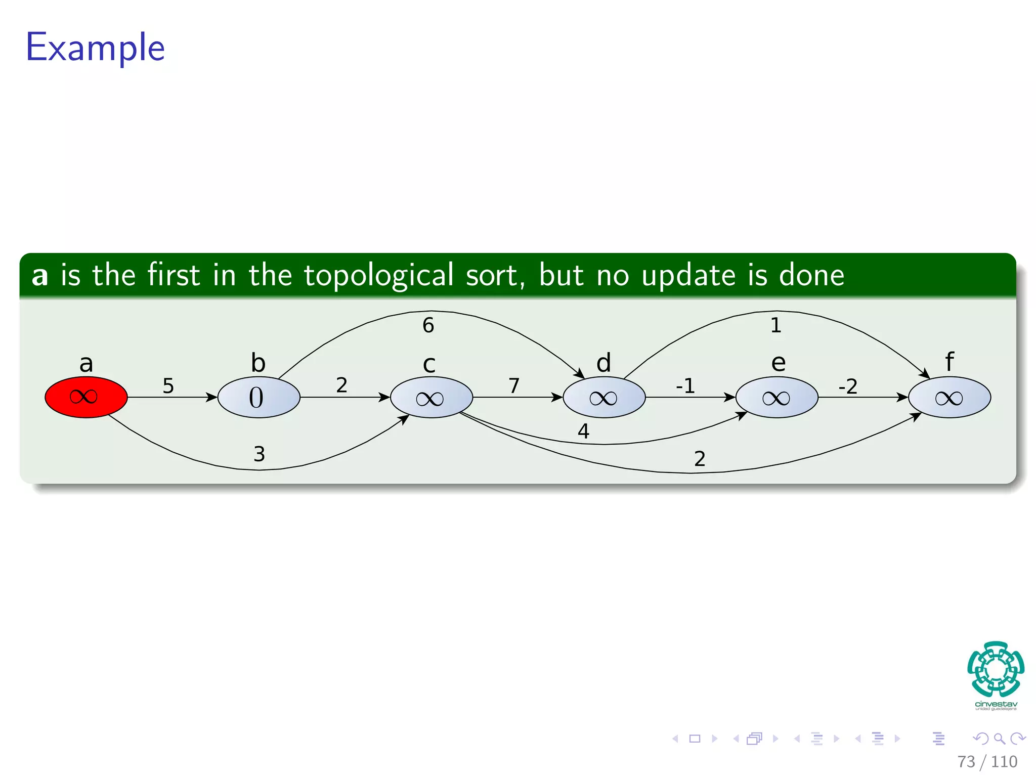
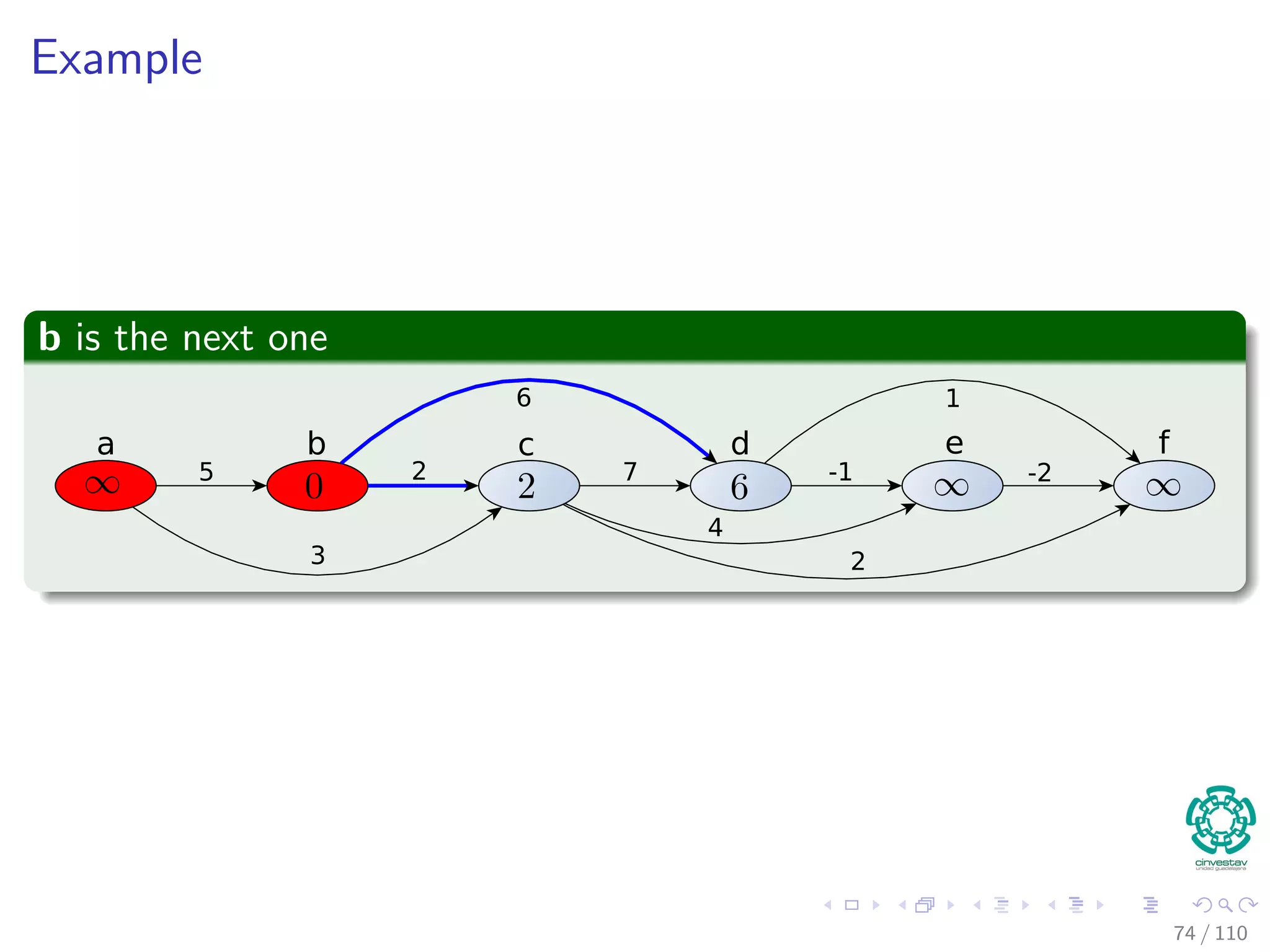
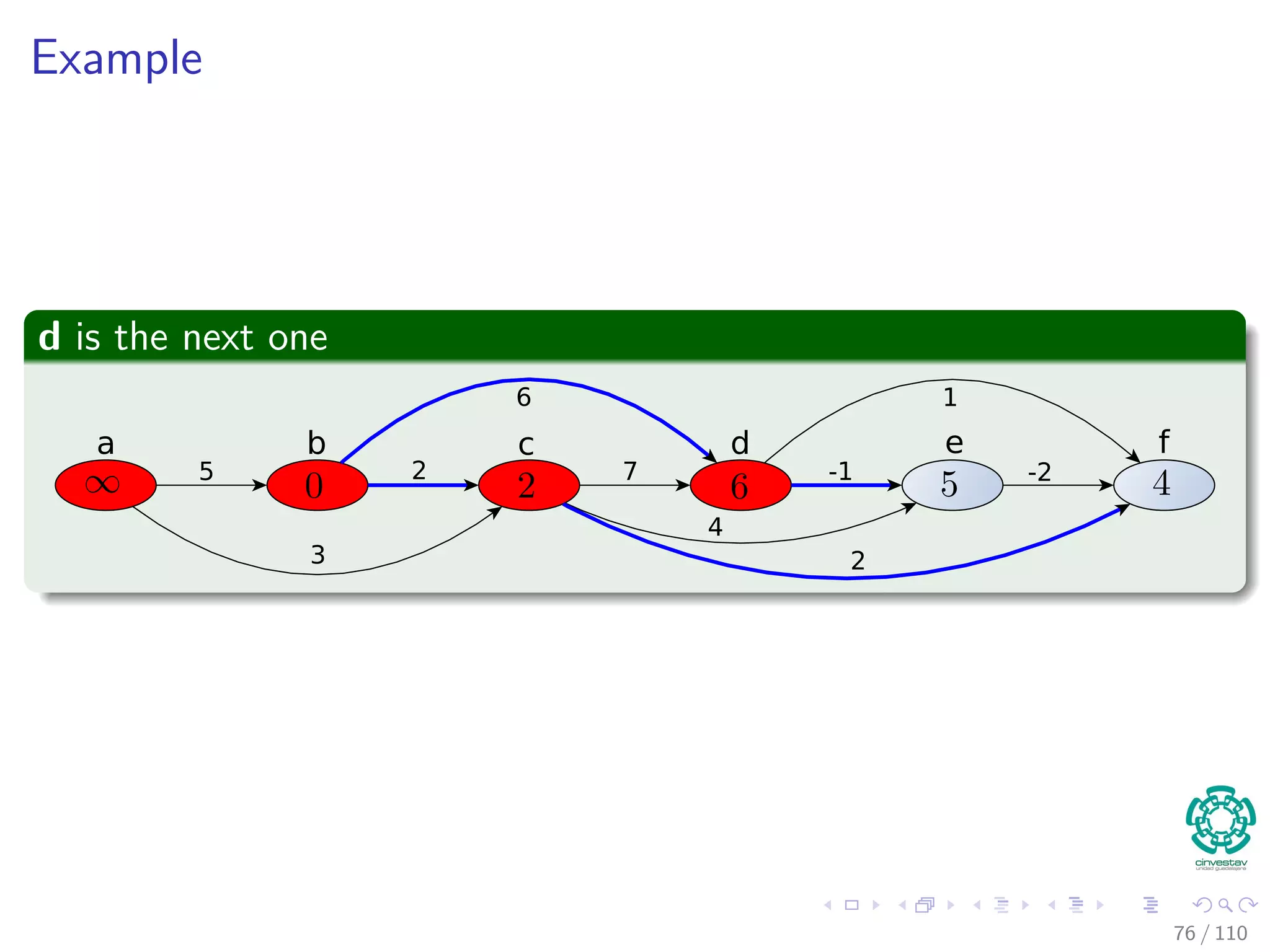
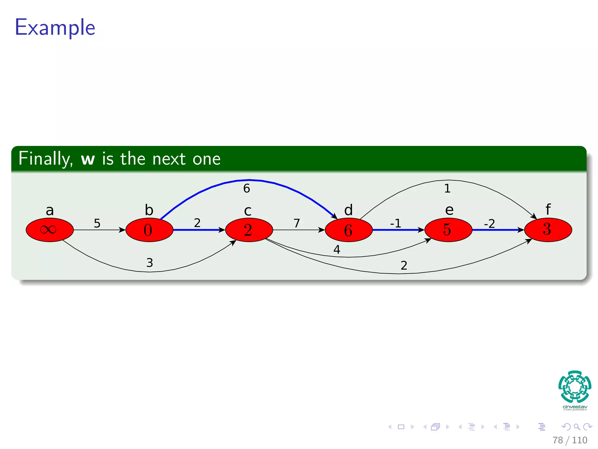
![Single-source Shortest Paths in Directed Acyclic Graphs
In a DAG, we can do the following (Complexity Θ (V + E))
DAG -SHORTEST-PATHS(G, w, s)
1 Topological sort vertices in G
2 Initialize(G, s)
3 for each u in V [G] in topological sorted order
4 for each v to Adj [u]
5 Relax(u, v, w)
66 / 108](https://image.slidesharecdn.com/20single-sourceshorthestpath-151109143432-lva1-app6891/75/20-Single-Source-Shorthest-Path-164-2048.jpg)
![Single-source Shortest Paths in Directed Acyclic Graphs
In a DAG, we can do the following (Complexity Θ (V + E))
DAG -SHORTEST-PATHS(G, w, s)
1 Topological sort vertices in G
2 Initialize(G, s)
3 for each u in V [G] in topological sorted order
4 for each v to Adj [u]
5 Relax(u, v, w)
66 / 108](https://image.slidesharecdn.com/20single-sourceshorthestpath-151109143432-lva1-app6891/75/20-Single-Source-Shorthest-Path-165-2048.jpg)
![Single-source Shortest Paths in Directed Acyclic Graphs
In a DAG, we can do the following (Complexity Θ (V + E))
DAG -SHORTEST-PATHS(G, w, s)
1 Topological sort vertices in G
2 Initialize(G, s)
3 for each u in V [G] in topological sorted order
4 for each v to Adj [u]
5 Relax(u, v, w)
66 / 108](https://image.slidesharecdn.com/20single-sourceshorthestpath-151109143432-lva1-app6891/75/20-Single-Source-Shorthest-Path-166-2048.jpg)


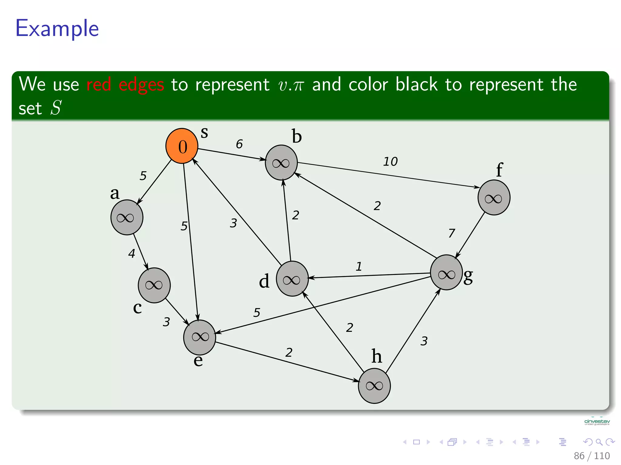
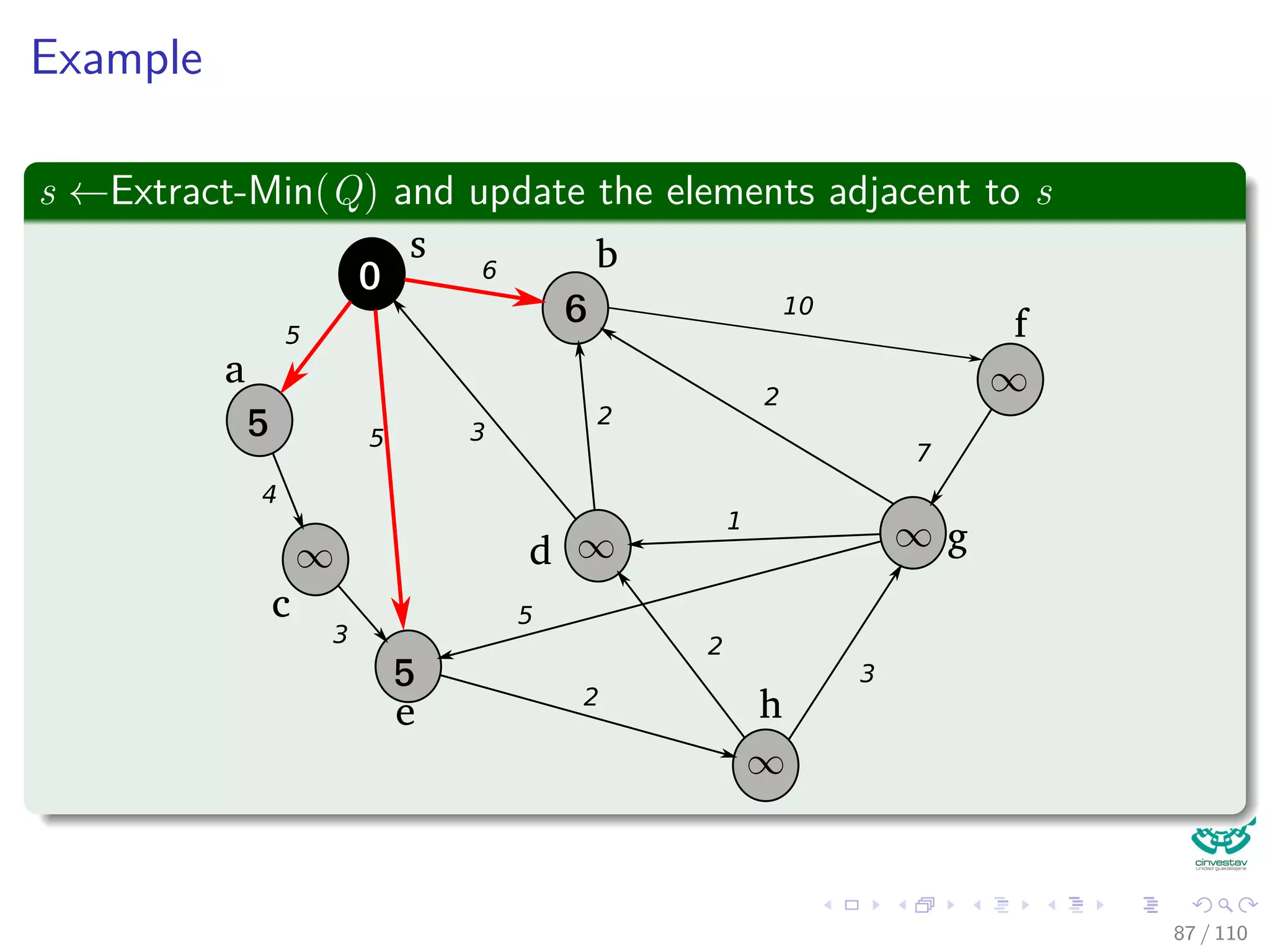

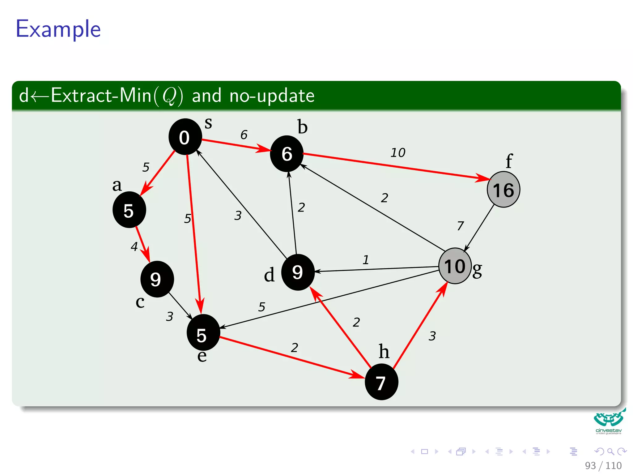
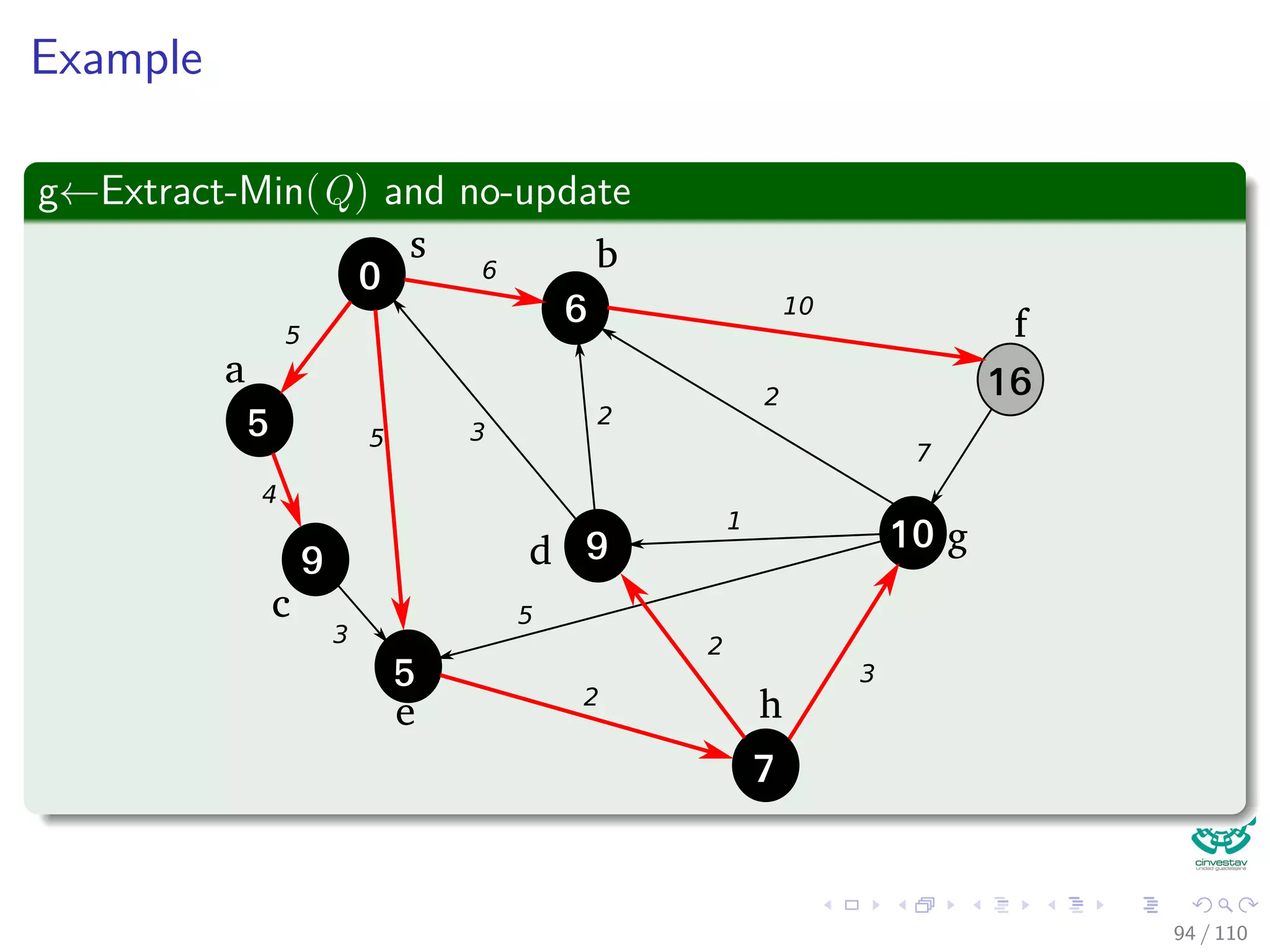
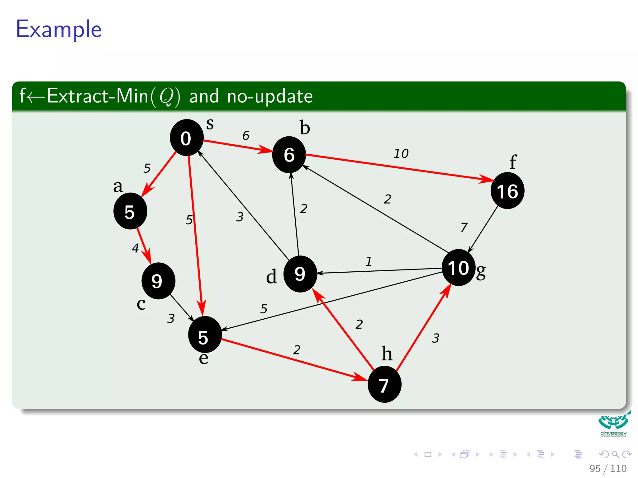
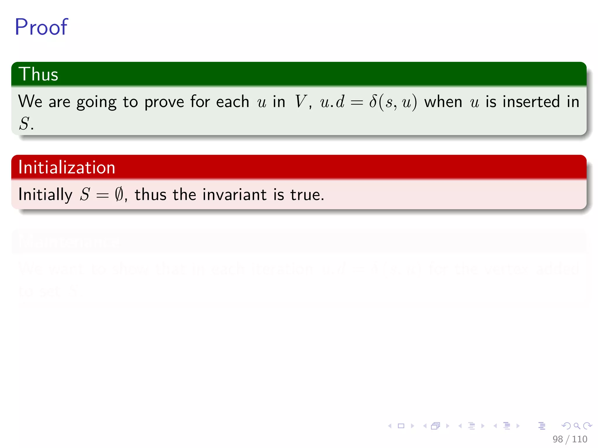
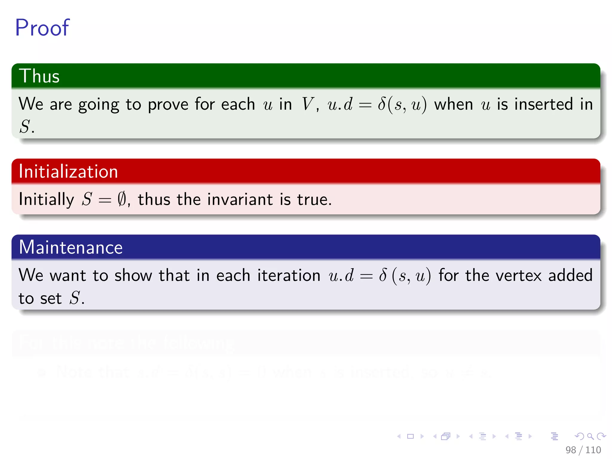
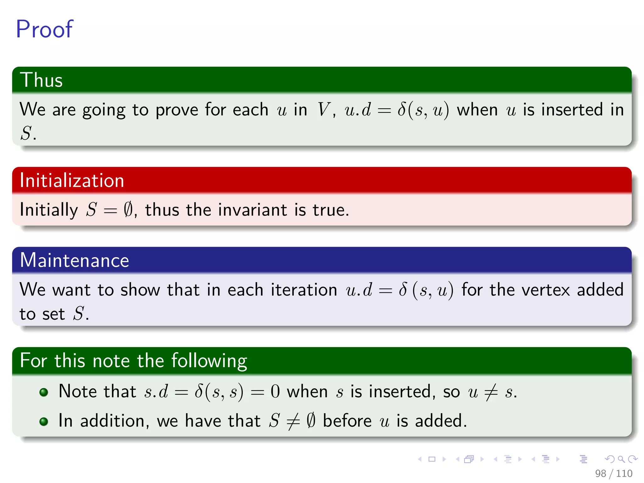
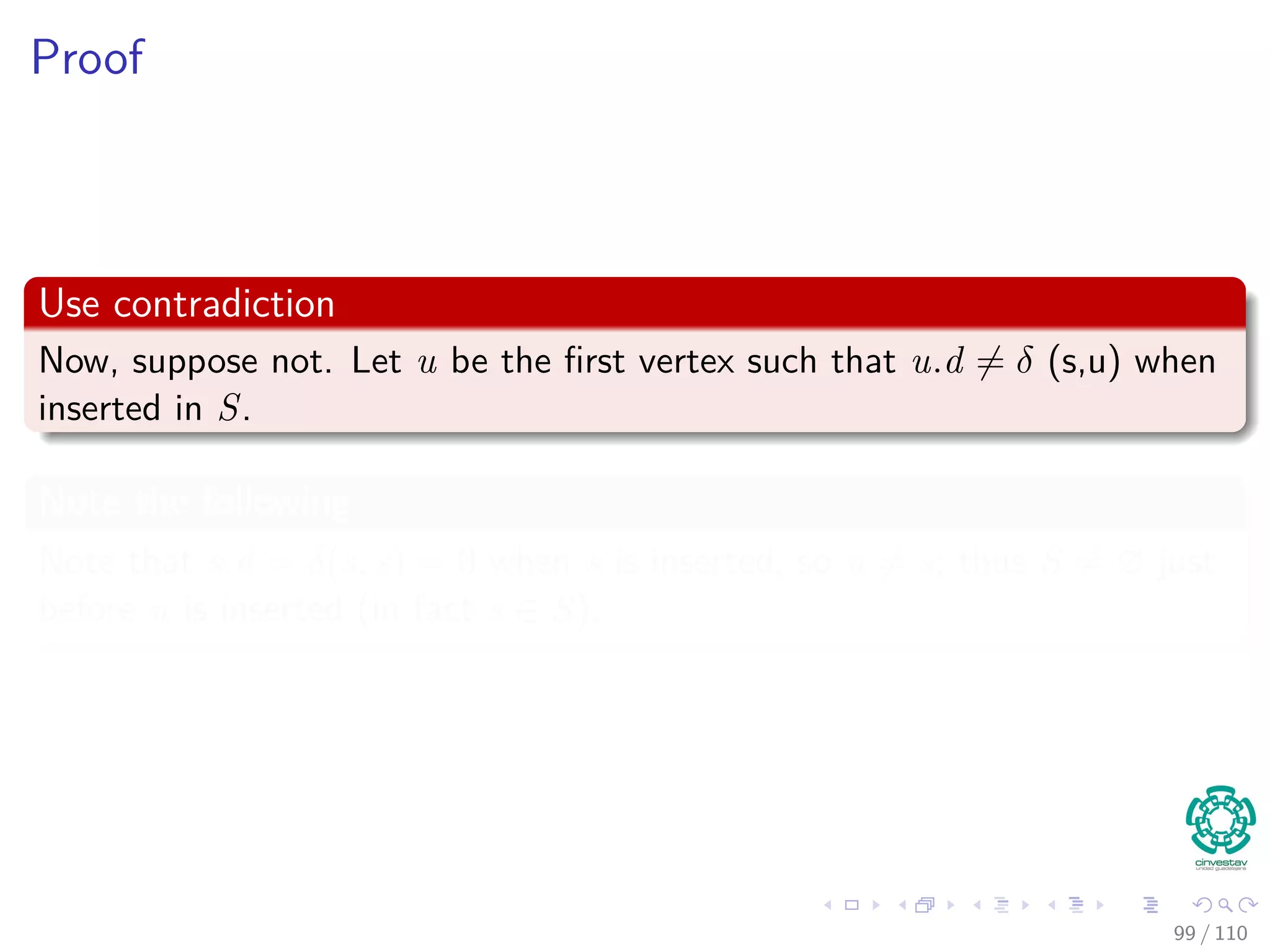
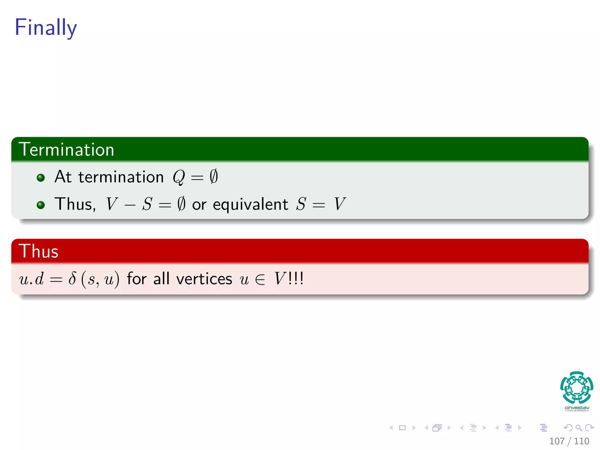
![Dijkstra’s algorithm
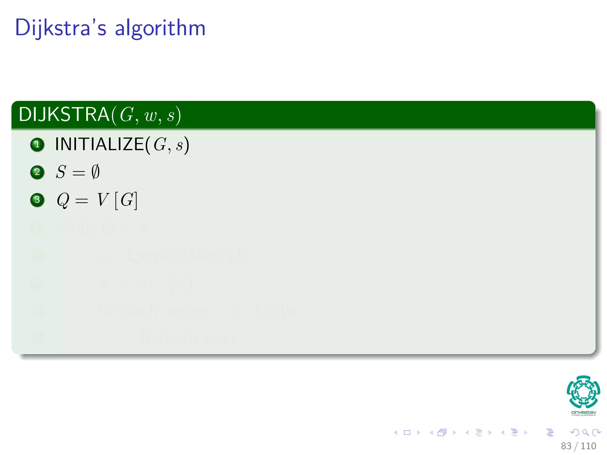
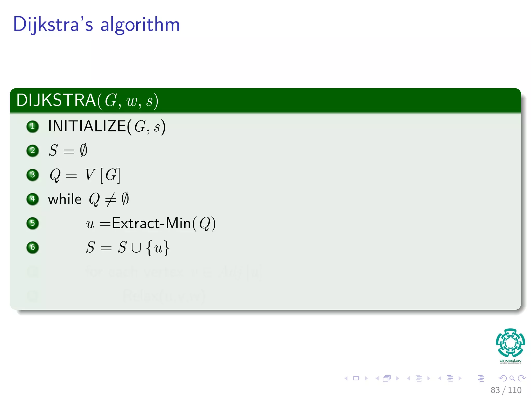
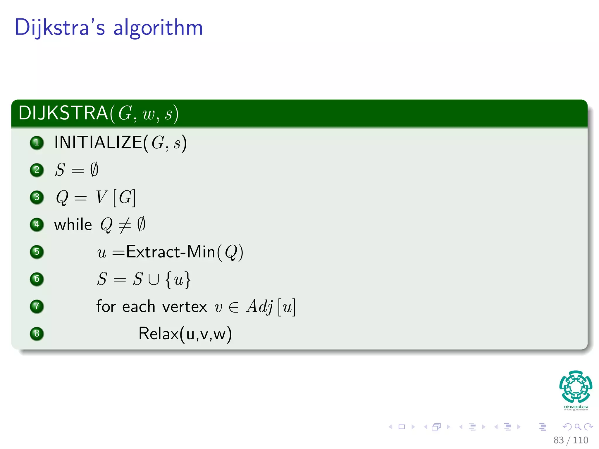
DIJKSTRA(G, w, s)
1 INITIALIZE(G, s)
2 S = ∅
3 Q = V [G]
4 while Q = ∅
5 u =Extract-Min(Q)
6 S = S ∪ {u}
7 for each vertex v ∈ Adj [u]
8 Relax(u,v,w)
80 / 108](https://image.slidesharecdn.com/20single-sourceshorthestpath-151109143432-lva1-app6891/75/20-Single-Source-Shorthest-Path-189-2048.jpg)
![Dijkstra’s algorithm
DIJKSTRA(G, w, s)
1 INITIALIZE(G, s)
2 S = ∅
3 Q = V [G]
4 while Q = ∅
5 u =Extract-Min(Q)
6 S = S ∪ {u}
7 for each vertex v ∈ Adj [u]
8 Relax(u,v,w)
80 / 108](https://image.slidesharecdn.com/20single-sourceshorthestpath-151109143432-lva1-app6891/75/20-Single-Source-Shorthest-Path-190-2048.jpg)
![Dijkstra’s algorithm
DIJKSTRA(G, w, s)
1 INITIALIZE(G, s)
2 S = ∅
3 Q = V [G]
4 while Q = ∅
5 u =Extract-Min(Q)
6 S = S ∪ {u}
7 for each vertex v ∈ Adj [u]
8 Relax(u,v,w)
80 / 108](https://image.slidesharecdn.com/20single-sourceshorthestpath-151109143432-lva1-app6891/75/20-Single-Source-Shorthest-Path-191-2048.jpg)


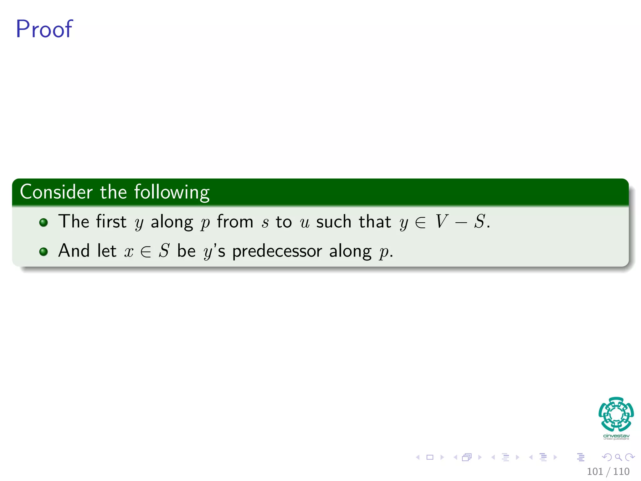
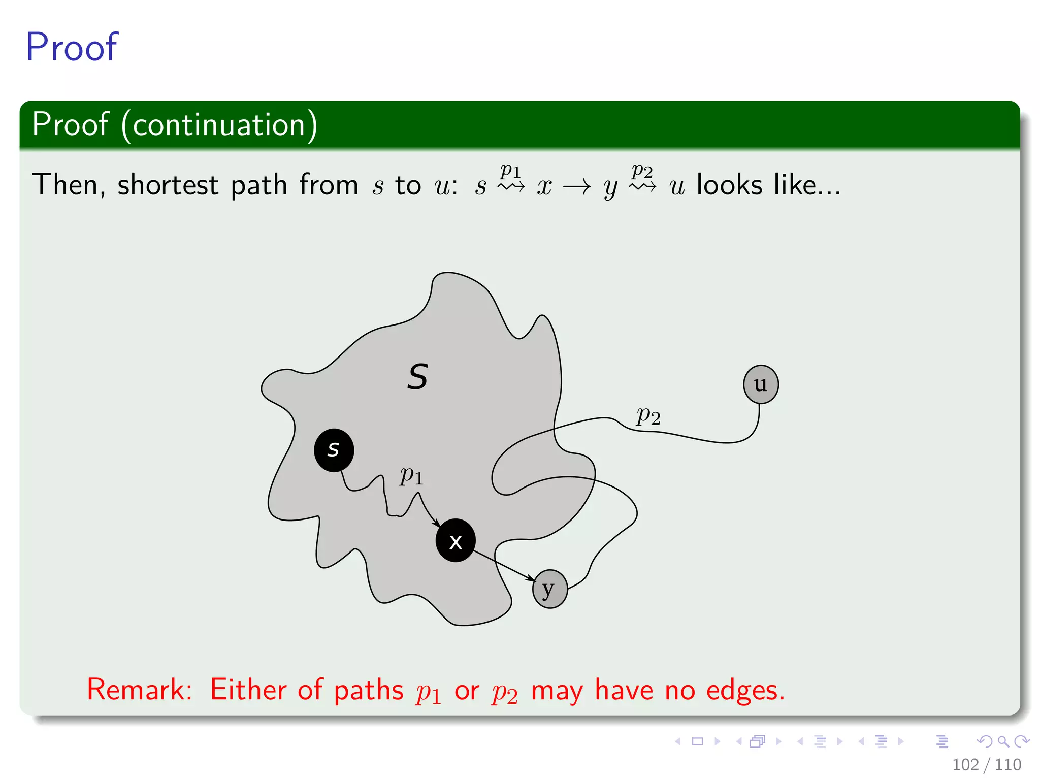

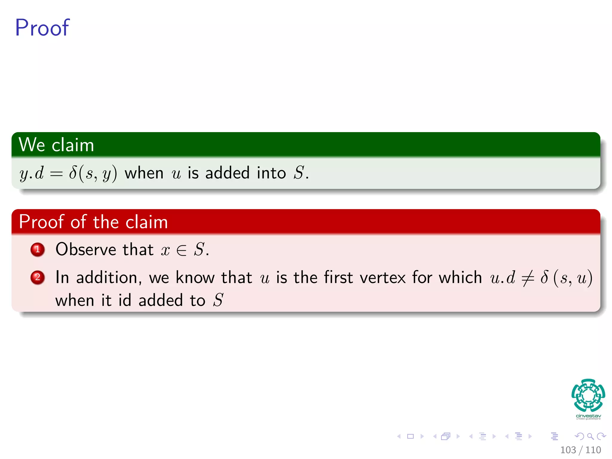
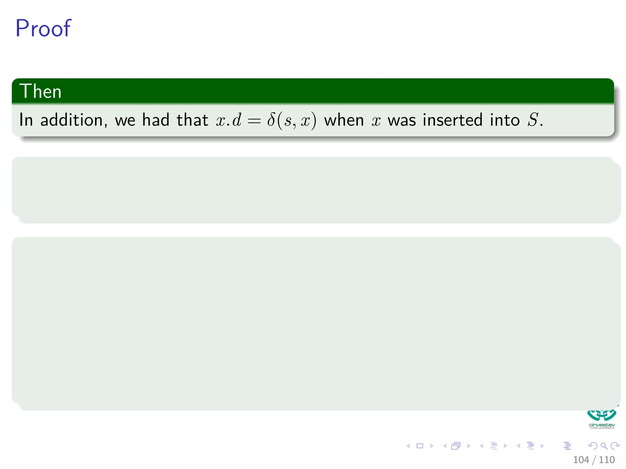


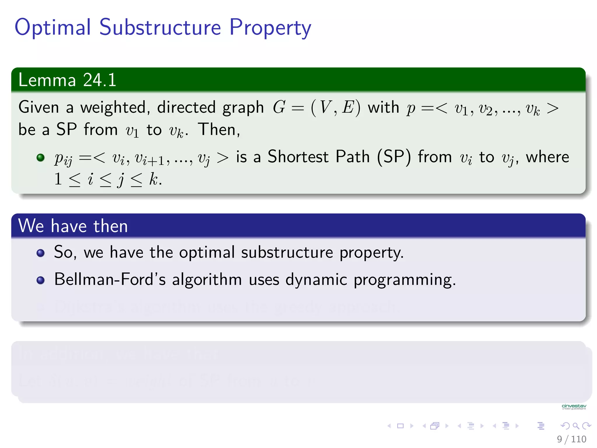
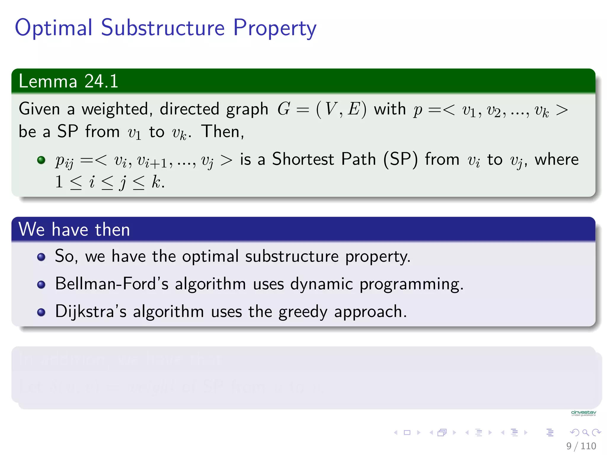
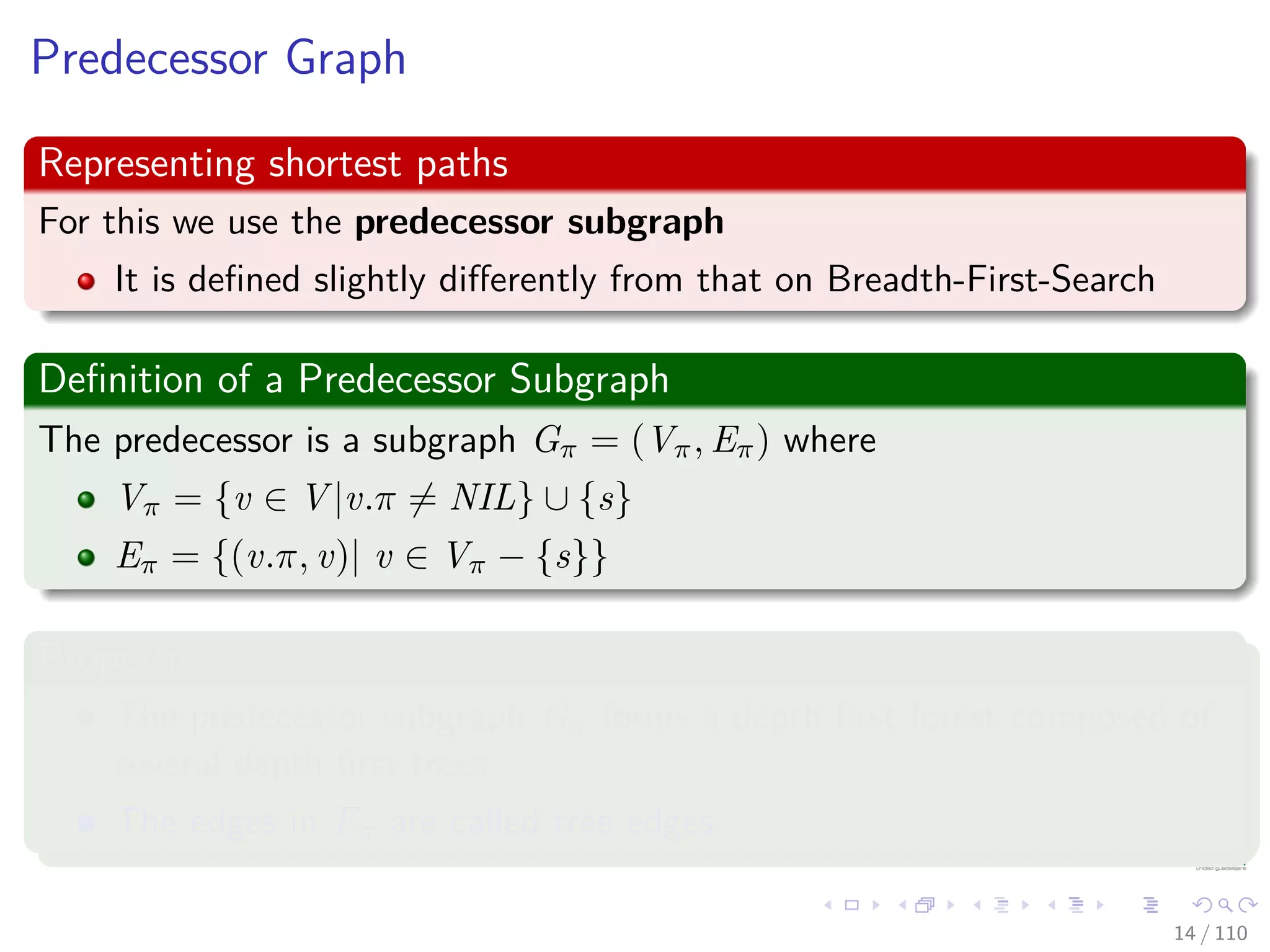
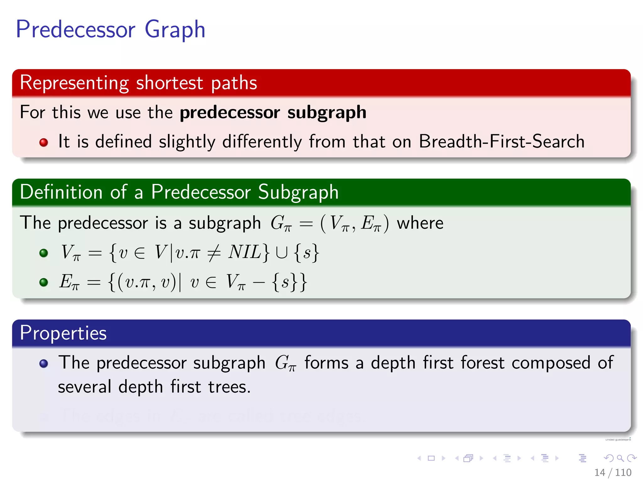
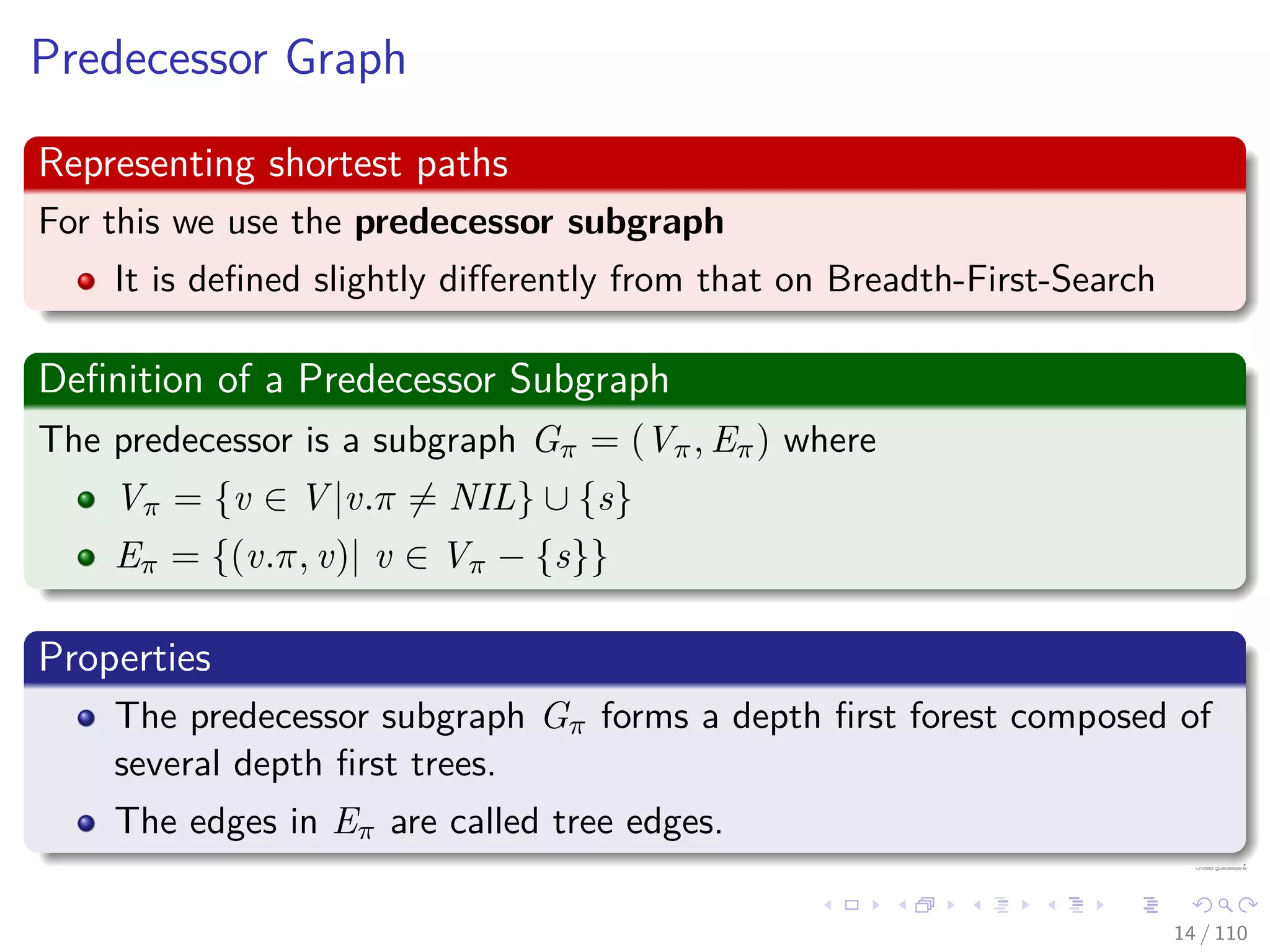
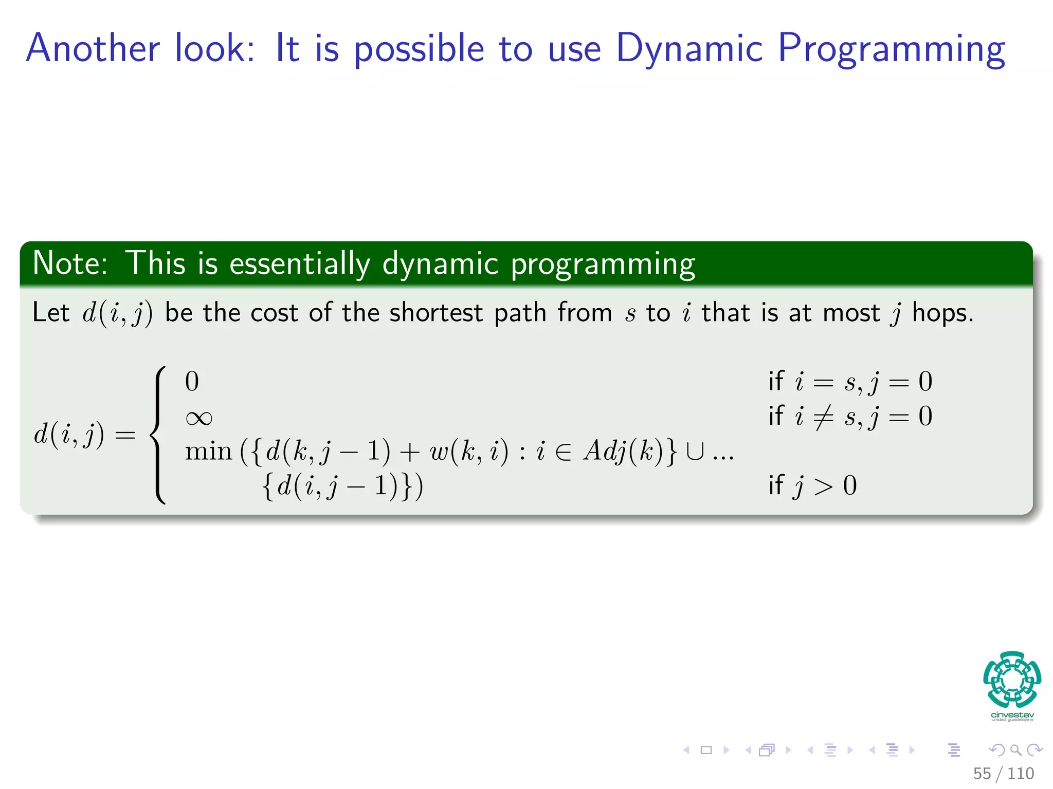
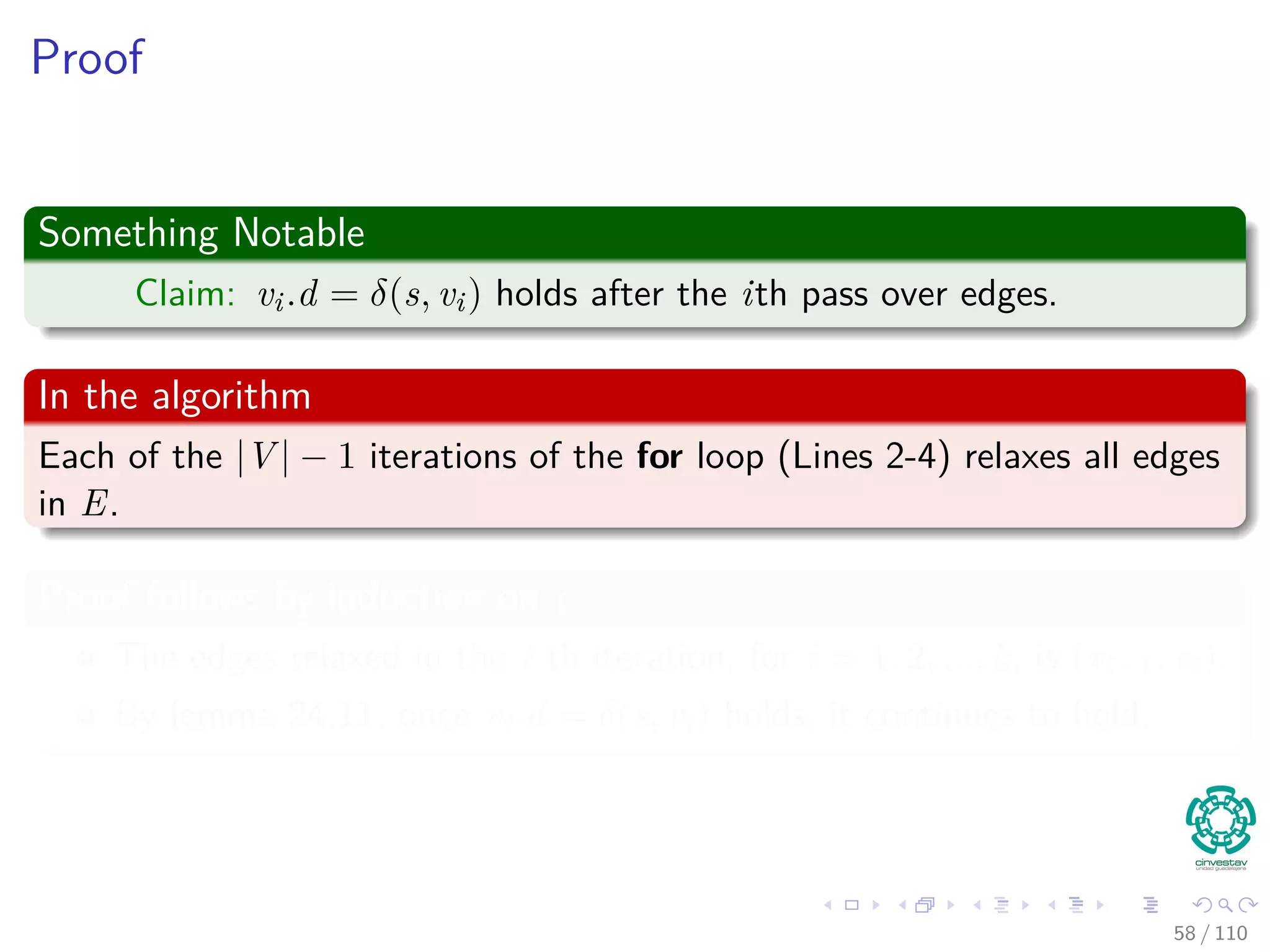
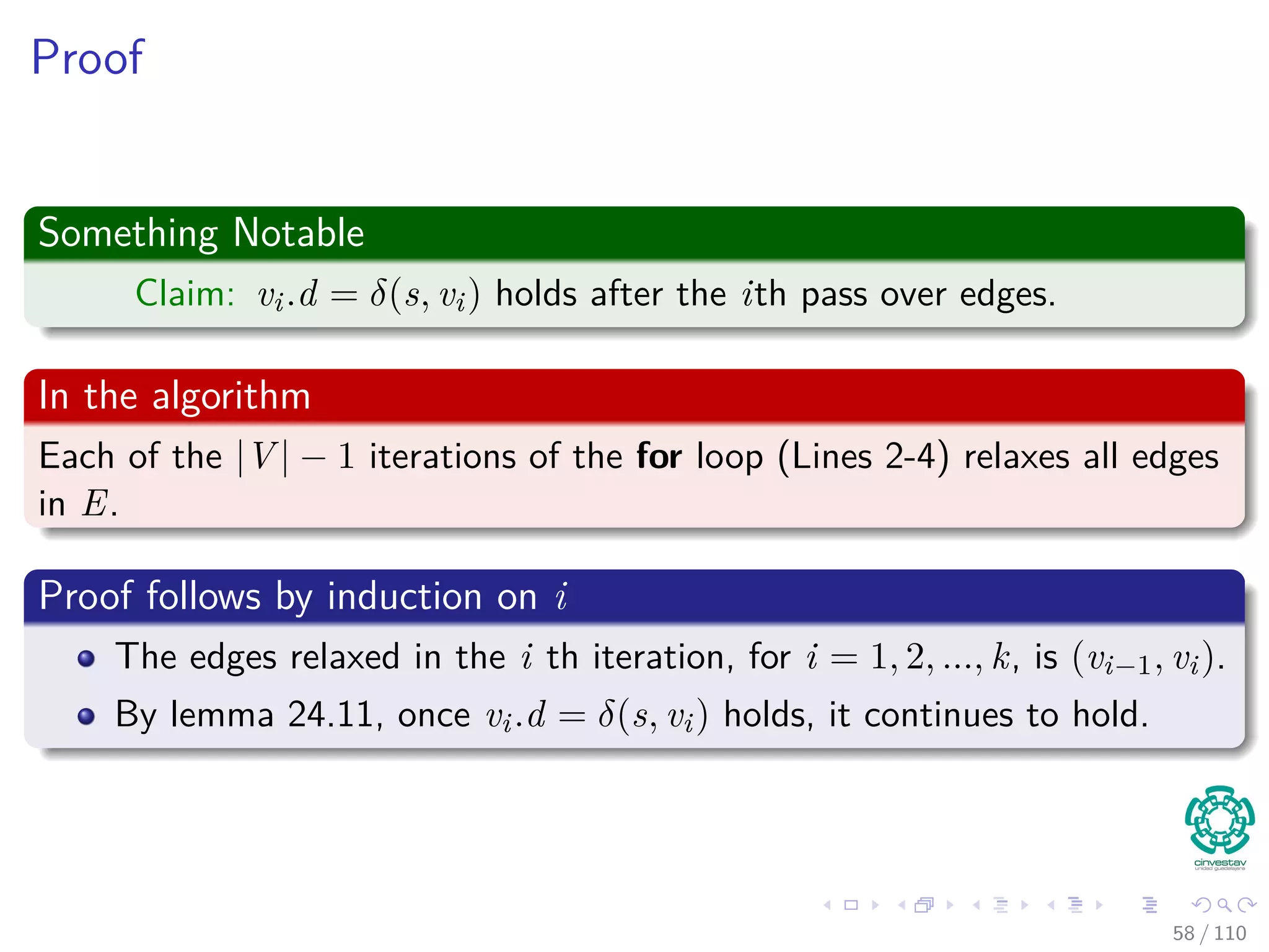
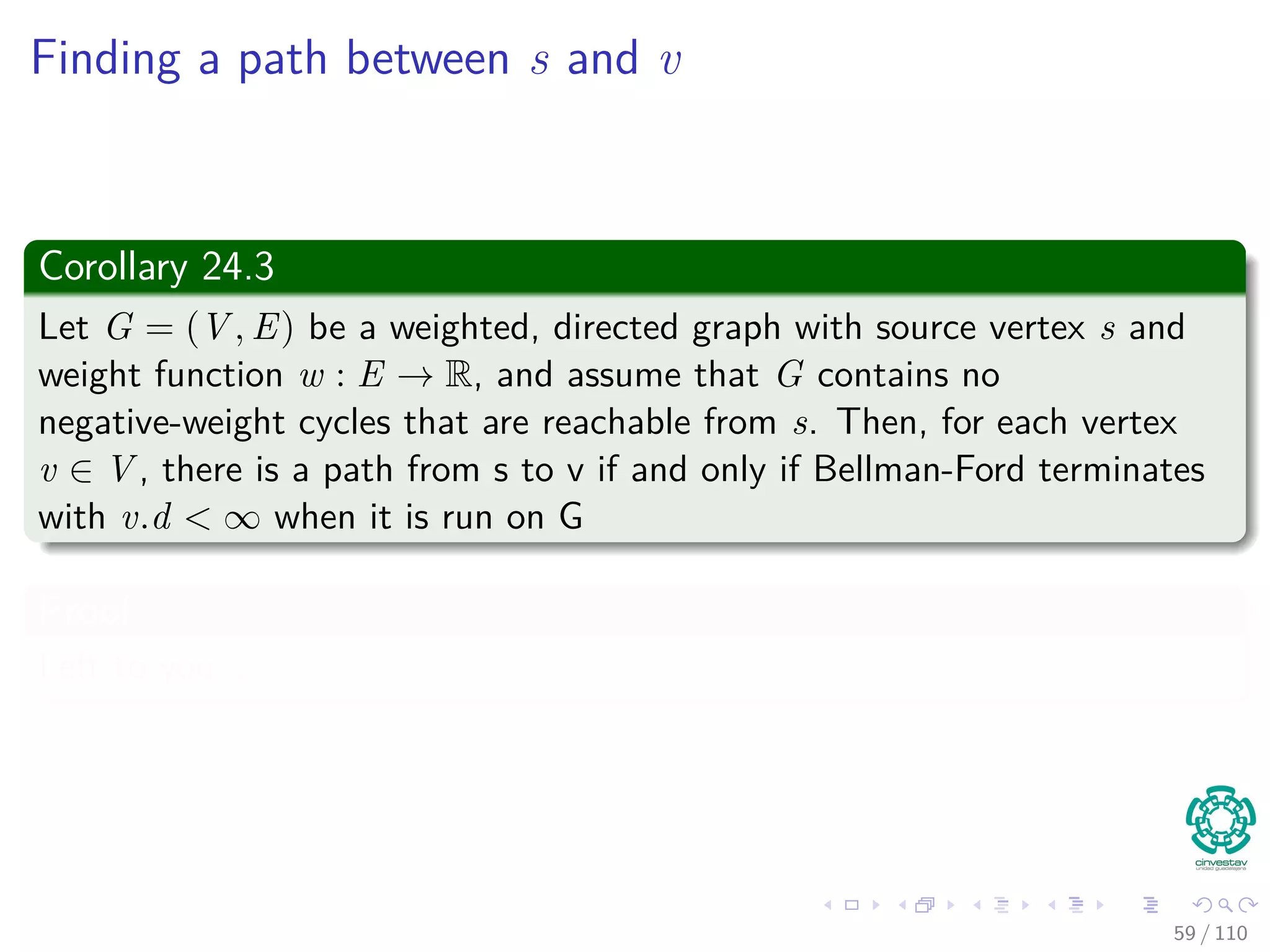
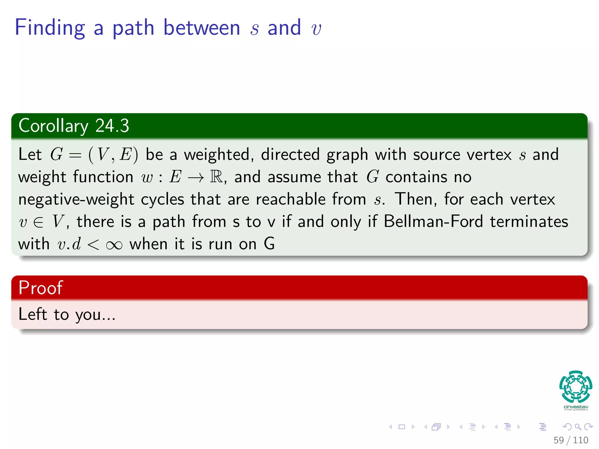
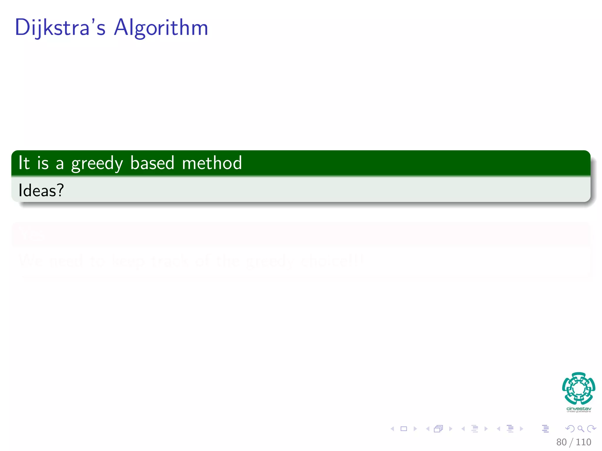
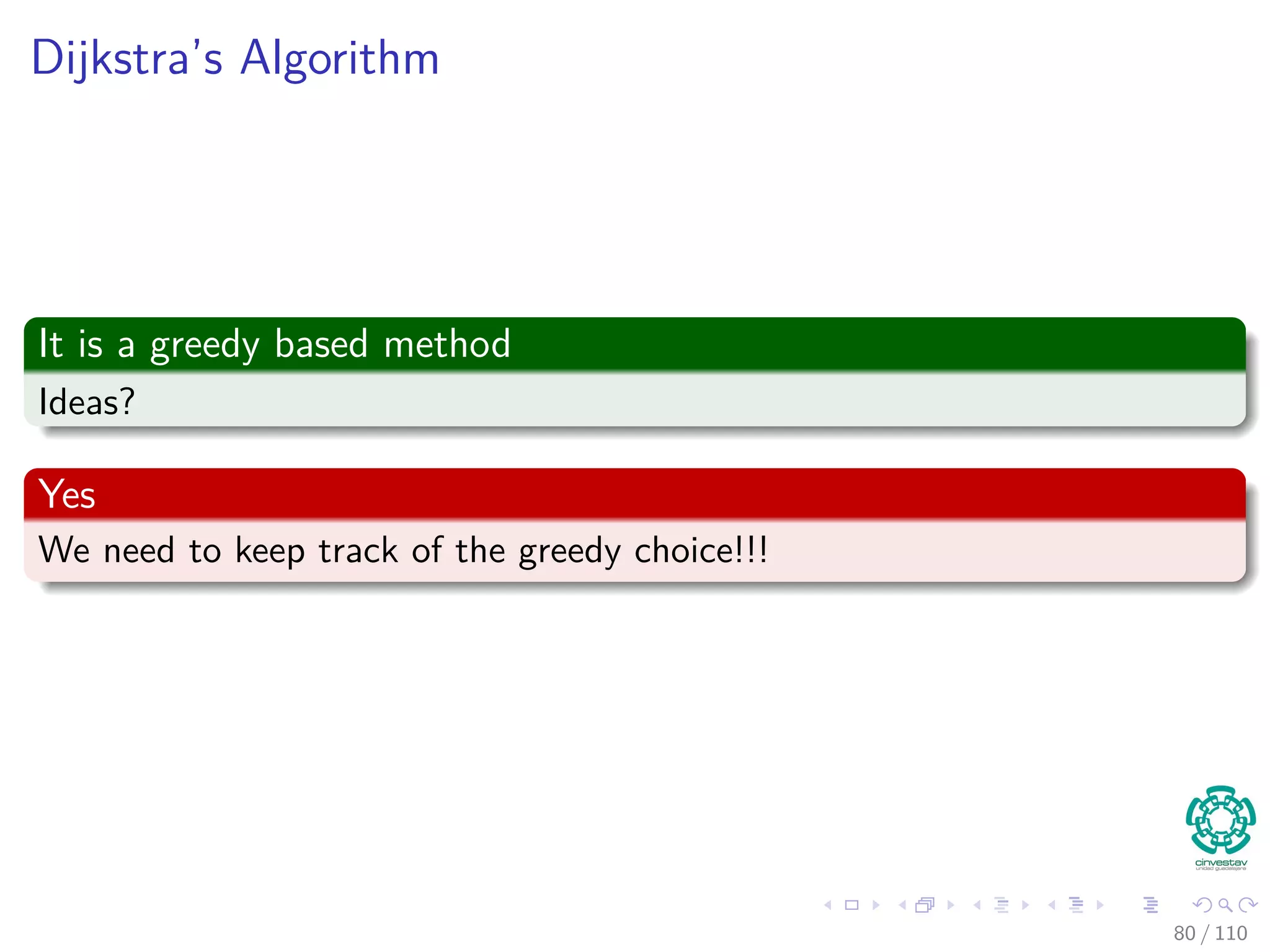
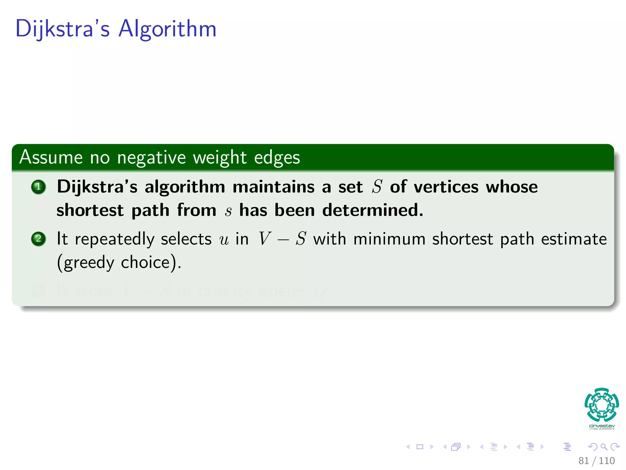
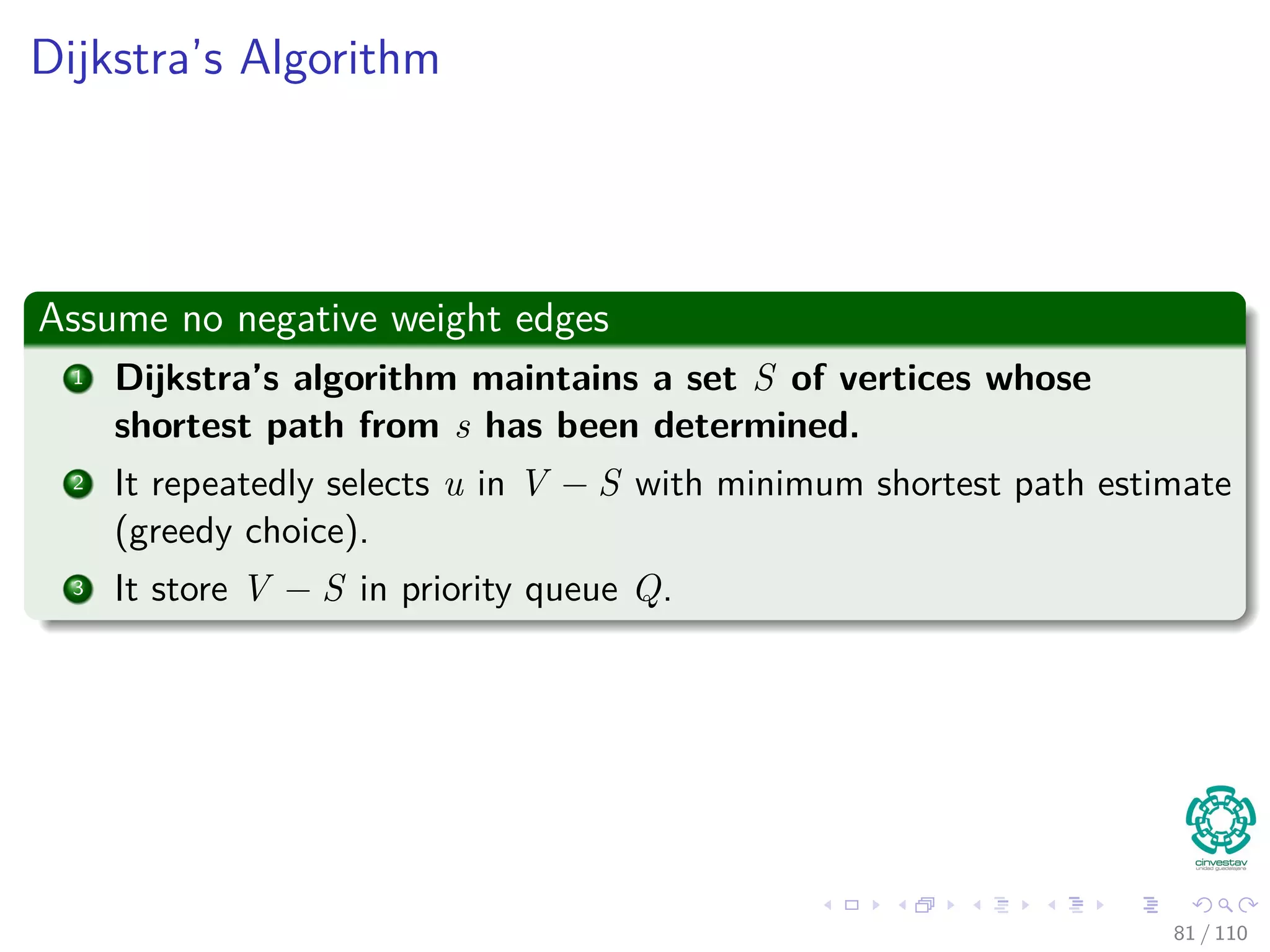
The document provides an in-depth analysis of algorithms for single-source shortest paths, focusing on the Bellman-Ford and Dijkstra's algorithms, and explains their mathematical foundations, such as optimal substructure and edge relaxation. It also discusses related problems, such as single destination and all pairs shortest paths, and outlines key concepts like predecessor graphs. The document emphasizes the capabilities of Bellman-Ford to handle negative weights and cycles, contrasting it with Dijkstra's greedy approach.


![ANPARA THERMAL POWER STATION[1] sangam.pdf](https://cdn.slidesharecdn.com/ss_thumbnails/anparathermalpowerstation1sangam-251121115219-9261cde4-thumbnail.jpg?width=640&height=640&fit=bounds)


