Download as PDF, PPTX


![For more on this...
Something Notable
As many things in the history of analysis of algorithms the all-pairs
shortest path has a long history.
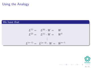
We have more from
“Studies in the Economics of Transportation” by Beckmann, McGuire, and
Winsten (1956) where the notation that we use for the matrix multiplication alike
was first used.
In addition
G. Tarry, Le probleme des labyrinthes, Nouvelles Annales de Mathématiques (3) 14 (1895)
187–190 [English translation in: N.L. Biggs, E.K. Lloyd, R.J. Wilson, Graph Theory
1736–1936, Clarendon Press, Oxford, 1976, pp. 18–20] (For the theory behind
depth-first search techniques).
Chr. Wiener, Ueber eine Aufgabe aus der Geometria situs, Mathematische Annalen 6
(1873) 29–30, 1873.
7 / 79](https://image.slidesharecdn.com/21allpairsshortestpath-151111121950-lva1-app6891/85/21-All-Pairs-Shortest-Path-18-320.jpg)
![For more on this...
Something Notable
As many things in the history of analysis of algorithms the all-pairs
shortest path has a long history.
We have more from
“Studies in the Economics of Transportation” by Beckmann, McGuire, and
Winsten (1956) where the notation that we use for the matrix multiplication alike
was first used.
In addition
G. Tarry, Le probleme des labyrinthes, Nouvelles Annales de Mathématiques (3) 14 (1895)
187–190 [English translation in: N.L. Biggs, E.K. Lloyd, R.J. Wilson, Graph Theory
1736–1936, Clarendon Press, Oxford, 1976, pp. 18–20] (For the theory behind
depth-first search techniques).
Chr. Wiener, Ueber eine Aufgabe aus der Geometria situs, Mathematische Annalen 6
(1873) 29–30, 1873.
7 / 79](https://image.slidesharecdn.com/21allpairsshortestpath-151111121950-lva1-app6891/85/21-All-Pairs-Shortest-Path-19-320.jpg)
![For more on this...
Something Notable
As many things in the history of analysis of algorithms the all-pairs
shortest path has a long history.
We have more from
“Studies in the Economics of Transportation” by Beckmann, McGuire, and
Winsten (1956) where the notation that we use for the matrix multiplication alike
was first used.
In addition
G. Tarry, Le probleme des labyrinthes, Nouvelles Annales de Mathématiques (3) 14 (1895)
187–190 [English translation in: N.L. Biggs, E.K. Lloyd, R.J. Wilson, Graph Theory
1736–1936, Clarendon Press, Oxford, 1976, pp. 18–20] (For the theory behind
depth-first search techniques).
Chr. Wiener, Ueber eine Aufgabe aus der Geometria situs, Mathematische Annalen 6
(1873) 29–30, 1873.
7 / 79](https://image.slidesharecdn.com/21allpairsshortestpath-151111121950-lva1-app6891/85/21-All-Pairs-Shortest-Path-20-320.jpg)
![For more on this...
Something Notable
As many things in the history of analysis of algorithms the all-pairs
shortest path has a long history.
We have more from
“Studies in the Economics of Transportation” by Beckmann, McGuire, and
Winsten (1956) where the notation that we use for the matrix multiplication alike
was first used.
In addition
G. Tarry, Le probleme des labyrinthes, Nouvelles Annales de Mathématiques (3) 14 (1895)
187–190 [English translation in: N.L. Biggs, E.K. Lloyd, R.J. Wilson, Graph Theory
1736–1936, Clarendon Press, Oxford, 1976, pp. 18–20] (For the theory behind
depth-first search techniques).
Chr. Wiener, Ueber eine Aufgabe aus der Geometria situs, Mathematische Annalen 6
(1873) 29–30, 1873.
7 / 79](https://image.slidesharecdn.com/21allpairsshortestpath-151111121950-lva1-app6891/85/21-All-Pairs-Shortest-Path-21-320.jpg)


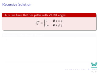


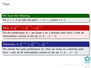
![Thus, we have the following
Recursive Version
Recursive-Floyd-Warshall(W )
1 D(n)
the n × n matrix
2 for i = 1 to n
3 for j = 1 to n
4 D(n)
[i, j] =Recursive-Part(i, j, n, W )
5 return D(n)
49 / 79](https://image.slidesharecdn.com/21allpairsshortestpath-151111121950-lva1-app6891/85/21-All-Pairs-Shortest-Path-98-320.jpg)
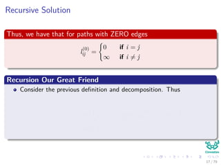
![Thus, we have the following
Recursive Version
Recursive-Floyd-Warshall(W )
1 D(n)
the n × n matrix
2 for i = 1 to n
3 for j = 1 to n
4 D(n)
[i, j] =Recursive-Part(i, j, n, W )
5 return D(n)
49 / 79](https://image.slidesharecdn.com/21allpairsshortestpath-151111121950-lva1-app6891/85/21-All-Pairs-Shortest-Path-99-320.jpg)
![Thus, we have the following
Recursive Version
Recursive-Floyd-Warshall(W )
1 D(n)
the n × n matrix
2 for i = 1 to n
3 for j = 1 to n
4 D(n)
[i, j] =Recursive-Part(i, j, n, W )
5 return D(n)
49 / 79](https://image.slidesharecdn.com/21allpairsshortestpath-151111121950-lva1-app6891/85/21-All-Pairs-Shortest-Path-100-320.jpg)
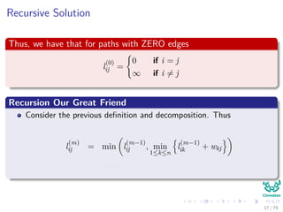
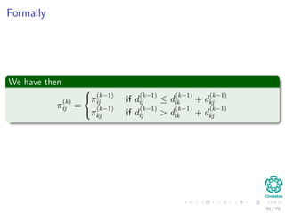
![Thus, we have the following
The Recursive-Part
Recursive-Part(i, j, k, W )
1 if k = 0
2 return W [i, j]
3 if k ≥ 1
4 t1 =Recursive-Part(i, j, k − 1, W )
5 t2 =Recursive-Part(i, k, k − 1, W )+...
6 Recursive-Part(k, j, k − 1, W )
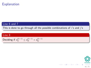
7 if t1 ≤ t2
8 return t1
9 else
10 return t2
50 / 79](https://image.slidesharecdn.com/21allpairsshortestpath-151111121950-lva1-app6891/85/21-All-Pairs-Shortest-Path-101-320.jpg)
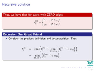
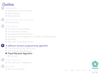
![Thus, we have the following
The Recursive-Part
Recursive-Part(i, j, k, W )
1 if k = 0
2 return W [i, j]
3 if k ≥ 1
4 t1 =Recursive-Part(i, j, k − 1, W )
5 t2 =Recursive-Part(i, k, k − 1, W )+...
6 Recursive-Part(k, j, k − 1, W )
7 if t1 ≤ t2
8 return t1
9 else
10 return t2
50 / 79](https://image.slidesharecdn.com/21allpairsshortestpath-151111121950-lva1-app6891/85/21-All-Pairs-Shortest-Path-102-320.jpg)
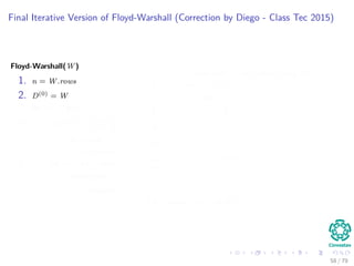
![Thus, we have the following
The Recursive-Part
Recursive-Part(i, j, k, W )
1 if k = 0
2 return W [i, j]
3 if k ≥ 1
4 t1 =Recursive-Part(i, j, k − 1, W )
5 t2 =Recursive-Part(i, k, k − 1, W )+...
6 Recursive-Part(k, j, k − 1, W )
7 if t1 ≤ t2
8 return t1
9 else
10 return t2
50 / 79](https://image.slidesharecdn.com/21allpairsshortestpath-151111121950-lva1-app6891/85/21-All-Pairs-Shortest-Path-103-320.jpg)
![Thus, we have the following
The Recursive-Part
Recursive-Part(i, j, k, W )
1 if k = 0
2 return W [i, j]
3 if k ≥ 1
4 t1 =Recursive-Part(i, j, k − 1, W )
5 t2 =Recursive-Part(i, k, k − 1, W )+...
6 Recursive-Part(k, j, k − 1, W )
7 if t1 ≤ t2
8 return t1
9 else
10 return t2
50 / 79](https://image.slidesharecdn.com/21allpairsshortestpath-151111121950-lva1-app6891/85/21-All-Pairs-Shortest-Path-104-320.jpg)


The document discusses the all-pairs shortest path problem, detailing various algorithms including Dijkstra's, Bellman-Ford, and the Floyd-Warshall algorithm. It emphasizes the problem's definition, assumptions, and provides insights on matrix representation and shortest path structures. The content further explores historical context and suggests exercises for practical understanding.