Elementary Graph Algorithms discusses graphs and common graph algorithms. It defines graphs as G = (V, E) with vertices V and edges E. It describes the breadth-first search (BFS) and depth-first search (DFS) algorithms. BFS expands the frontier between discovered and undiscovered vertices uniformly across the breadth of the frontier. It uses a queue and runs in O(V+E) time. DFS explores edges out of the most recently discovered vertex, searching as deep as possible first before backtracking. It uses timestamps and runs in O(V+E) time. Pseudocode and examples are provided for both algorithms.

1. Elementary Graph Algorithms
Dr. AMIT KUMAR @JUET

2. Graphs
• Graph G = (V, E)
– V = set of vertices
– E = set of edges  (VV)
• Types of graphs
– Undirected: edge (u, v) = (v, u); for all v, (v, v)  E (No self loops.)
– Directed: (u, v) is edge from u to v, denoted as u  v. Self loops
are allowed.
– Weighted: each edge has an associated weight, given by a weight
function w : E  R.
– Dense: |E|  |V|2.
– Sparse: |E| << |V|2.
• |E| = O(|V|2)
Dr. AMIT KUMAR @JUET

3. Graphs
• If (u, v)  E, then vertex v is adjacent to vertex u.
• Adjacency relationship is:
– Symmetric if G is undirected.
– Not necessarily so if G is directed.
• If G is connected:
– There is a path between every pair of vertices.
– |E|  |V| – 1.
– Furthermore, if |E| = |V| – 1, then G is a tree.
• Other definitions in Appendix B (B.4 and B.5) as needed.
Dr. AMIT KUMAR @JUET

4. Representation of Graphs
• Two standard ways.
– Adjacency Lists.
– Adjacency Matrix.
a
dc
b a
b
c
d
b
a
d
d c
c
a b
a c
a
dc
b
1 2
3 4
1 2 3 4
1 0 1 1 1
2 1 0 1 0
3 1 1 0 1
4 1 0 1 0
Dr. AMIT KUMAR @JUET

5. Adjacency Lists
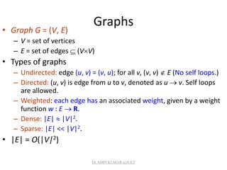
• Consists of an array Adj of |V| lists.
• One list per vertex.
• For u  V, Adj[u] consists of all vertices adjacent to u.
a
dc
b a
b
c
d
b
c
d
d c
a
dc
b a
b
c
d
b
a
d
d c
c
a b
a c
If weighted, store weights also in
adjacency lists.
Dr. AMIT KUMAR @JUET

6. Storage Requirement
• For directed graphs:
– Sum of lengths of all adj. lists is
out-degree(v) = |E|
vV
– Total storage: (V+E)
• For undirected graphs:
– Sum of lengths of all adj. lists is
degree(v) = 2|E|
vV
– Total storage: (V+E)
No. of edges leaving v
No. of edges incident on v. Edge (u,v) is incident
on vertices u and v.
Dr. AMIT KUMAR @JUET

7. Pros and Cons: adj list
• Pros
– Space-efficient, when a graph is sparse.
– Can be modified to support many graph variants.
• Cons
– Determining if an edge (u,v) G is not efficient.
• Have to search in u’s adjacency list. (degree(u)) time.
• (V) in the worst case.
Dr. AMIT KUMAR @JUET

8. Adjacency Matrix
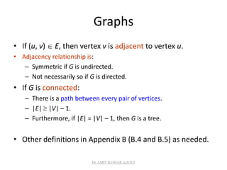
• |V|  |V| matrix A.
• Number vertices from 1 to |V| in some arbitrary
manner.
• A is then given by:


 

otherwise0
),(if1
],[
Eji
ajiA ij
a
dc
b
1 2
3 4
1 2 3 4
1 0 1 1 1
2 0 0 1 0
3 0 0 0 1
4 0 0 0 0
a
dc
b
1 2
3 4
1 2 3 4
1 0 1 1 1
2 1 0 1 0
3 1 1 0 1
4 1 0 1 0
A = AT for undirected graphs.
Dr. AMIT KUMAR @JUET

9. Space and Time
• Space: (V2).
– Not memory efficient for large graphs.
• Time: to list all vertices adjacent to u: (V).
• Time: to determine if (u, v)  E: (1).
• Can store weights instead of bits for weighted graph.
Dr. AMIT KUMAR @JUET

10. Graph-searching Algorithms
• Searching a graph:
– Systematically follow the edges of a graph
to visit the vertices of the graph.
• Used to discover the structure of a graph.
• Standard graph-searching algorithms.
– Breadth-first Search (BFS).
– Depth-first Search (DFS).
Dr. AMIT KUMAR @JUET

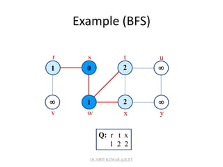
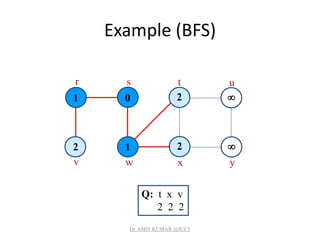
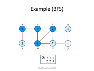
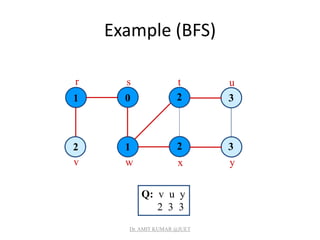
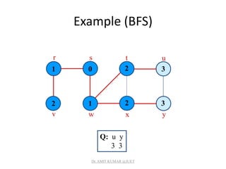
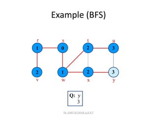
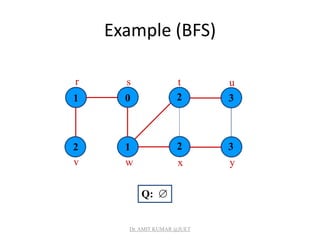
11. Breadth-first Search
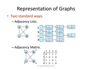
• Input: Graph G = (V, E), either directed or undirected,
and source vertex s  V.
• Output:
– d[v] = distance (smallest # of edges, or shortest path) from s to
v, for all v  V. d[v] =  if v is not reachable from s.
– [v] = u such that (u, v) is last edge on shortest path s v.
• u is v’s predecessor.
– Builds breadth-first tree with root s that contains all reachable
vertices.
Definitions:
Path between vertices u and v: Sequence of vertices (v1, v2, …, vk) such that
u=v1 and v =vk, and (vi,vi+1)  E, for all 1 i  k-1.
Length of the path: Number of edges in the path.
Path is simple if no vertex is repeated.
Error!
Dr. AMIT KUMAR @JUET

12. Breadth-first Search
• Expands the frontier between discovered and
undiscovered vertices uniformly across the breadth of
the frontier.
– A vertex is “discovered” the first time it is encountered during
the search.
– A vertex is “finished” if all vertices adjacent to it have been
discovered.
• Colors the vertices to keep track of progress.
– White – Undiscovered.
– Gray – Discovered but not finished.
– Black – Finished.
• Colors are required only to reason about the algorithm. Can be
implemented without colors.
Dr. AMIT KUMAR @JUET

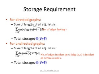
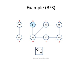
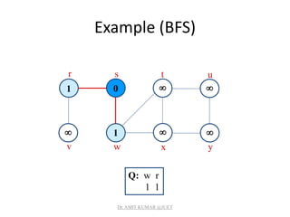
13. BFS(G,s)
1. for each vertex u in V[G] – {s}
2 do color[u]  white
3 d[u]  
4 [u]  nil
5 color[s]  gray
6 d[s]  0
7 [s]  nil
8 Q  
9 enqueue(Q,s)
10 while Q  
11 do u  dequeue(Q)
12 for each v in Adj[u]
13 do if color[v] = white
14 then color[v]  gray
15 d[v]  d[u] + 1
16 [v]  u
17 enqueue(Q,v)
18 color[u]  black
white: undiscovered
gray: discovered
black: finished
Q: a queue of discovered
vertices
color[v]: color of v
d[v]: distance from s to v
[u]: predecessor of v
Example: animation.
Dr. AMIT KUMAR @JUET

14. Example (BFS)
 0
  
 

r s t u
v w x y
Q: s
0
Dr. AMIT KUMAR @JUET

15. Example (BFS)
1 0
1  
 

r s t u
v w x y
Q: w r
1 1
Dr. AMIT KUMAR @JUET

16. Example (BFS)
1 0
1 2 
2 

r s t u
v w x y
Q: r t x
1 2 2
Dr. AMIT KUMAR @JUET

17. Example (BFS)
1 0
1 2 
2 
2
r s t u
v w x y
Q: t x v
2 2 2
Dr. AMIT KUMAR @JUET

18. Example (BFS)
1 0
1 2 
2 3
2
r s t u
v w x y
Q: x v u
2 2 3
Dr. AMIT KUMAR @JUET

19. Example (BFS)
1 0
1 2 3
2 3
2
r s t u
v w x y
Q: v u y
2 3 3
Dr. AMIT KUMAR @JUET

20. Example (BFS)
1 0
1 2 3
2 3
2
r s t u
v w x y
Q: u y
3 3
Dr. AMIT KUMAR @JUET

21. Example (BFS)
1 0
1 2 3
2 3
2
r s t u
v w x y
Q: y
3
Dr. AMIT KUMAR @JUET

22. Example (BFS)
1 0
1 2 3
2 3
2
r s t u
v w x y
Q: 
Dr. AMIT KUMAR @JUET

23. Example (BFS)
1 0
1 2 3
2 3
2
r s t u
v w x y
BF Tree
Dr. AMIT KUMAR @JUET

24. Analysis of BFS
• Initialization takes O(V).
• Traversal Loop
– After initialization, each vertex is enqueued and dequeued at
most once, and each operation takes O(1). So, total time for
queuing is O(V).
– The adjacency list of each vertex is scanned at most once. The
sum of lengths of all adjacency lists is (E).
• Summing up over all vertices => total running time of BFS
is O(V+E), linear in the size of the adjacency list
representation of graph.
• Correctness Proof
– We omit for BFS and DFS.
– Will do for later algorithms.
Dr. AMIT KUMAR @JUET

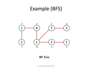
25. Breadth-first Tree
• For a graph G = (V, E) with source s, the predecessor
subgraph of G is G = (V , E) where
– V ={vV : [v]  NIL}{s}
– E ={([v],v)E : v  V - {s}}
• The predecessor subgraph G is a breadth-first tree if:
– V consists of the vertices reachable from s and
– for all vV , there is a unique simple path from s to v in G
that is also a shortest path from s to v in G.
• The edges in E are called tree edges.
|E | = |V | - 1.
Dr. AMIT KUMAR @JUET

26. Depth-first Search (DFS)
• Explore edges out of the most recently discovered
vertex v.
• When all edges of v have been explored, backtrack to
explore other edges leaving the vertex from which v
was discovered (its predecessor).
• “Search as deep as possible first.”
• Continue until all vertices reachable from the original
source are discovered.
• If any undiscovered vertices remain, then one of them
is chosen as a new source and search is repeated from
that source.
Dr. AMIT KUMAR @JUET

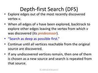
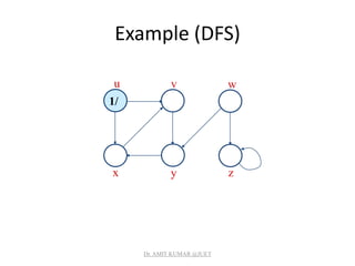
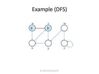
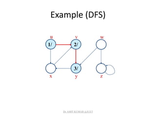
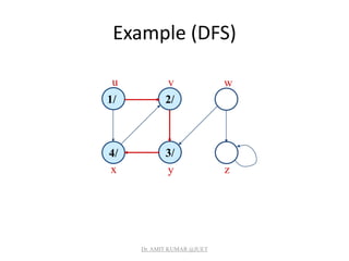
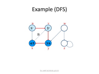
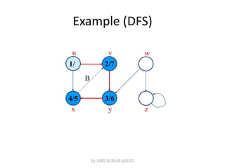
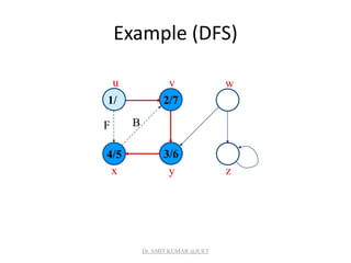
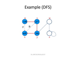
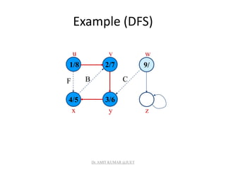
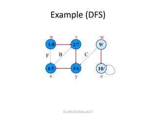
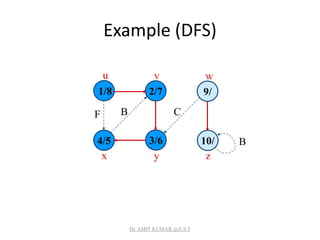
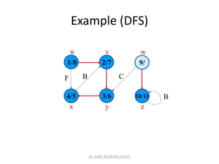
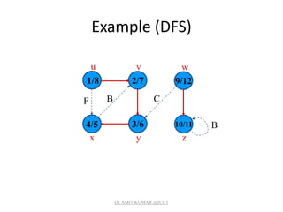
27. Depth-first Search
• Input: G = (V, E), directed or undirected. No source
vertex given!
• Output:
– 2 timestamps on each vertex. Integers between 1 and 2|V|.
• d[v] = discovery time (v turns from white to gray)
• f [v] = finishing time (v turns from gray to black)
– [v] : predecessor of v = u, such that v was discovered during
the scan of u’s adjacency list.
• Uses the same coloring scheme for vertices as BFS.
Dr. AMIT KUMAR @JUET

28. Pseudo-code
DFS(G)
1. for each vertex u  V[G]
2. do color[u]  white
3. [u]  NIL
4. time  0
5. for each vertex u  V[G]
6. do if color[u] = white
7. then DFS-Visit(u)
Uses a global timestamp time.
DFS-Visit(u)
1. color[u]  GRAY  White vertex u
has been discovered
2. time  time + 1
3. d[u]  time
4. for each v  Adj[u]
5. do if color[v] = WHITE
6. then [v]  u
7. DFS-Visit(v)
8. color[u]  BLACK  Blacken u;
it is finished.
9. f[u]  time  time + 1
Dr. AMIT KUMAR @JUET

29. Example (DFS)
1/
u v w
x y z
Dr. AMIT KUMAR @JUET

30. Example (DFS)
1/ 2/
u v w
x y z
Dr. AMIT KUMAR @JUET

31. Example (DFS)
1/
3/
2/
u v w
x y z
Dr. AMIT KUMAR @JUET

32. Example (DFS)
1/
4/ 3/
2/
u v w
x y z
Dr. AMIT KUMAR @JUET

33. Example (DFS)
1/
4/ 3/
2/
u v w
x y z
B
Dr. AMIT KUMAR @JUET

34. Example (DFS)
1/
4/5 3/
2/
u v w
x y z
B
Dr. AMIT KUMAR @JUET

35. Example (DFS)
1/
4/5 3/6
2/
u v w
x y z
B
Dr. AMIT KUMAR @JUET

36. Example (DFS)
1/
4/5 3/6
2/7
u v w
x y z
B
Dr. AMIT KUMAR @JUET

37. Example (DFS)
1/
4/5 3/6
2/7
u v w
x y z
BF
Dr. AMIT KUMAR @JUET

38. Example (DFS)
1/8
4/5 3/6
2/7
u v w
x y z
BF
Dr. AMIT KUMAR @JUET

39. Example (DFS)
1/8
4/5 3/6
2/7 9/
u v w
x y z
BF
Dr. AMIT KUMAR @JUET

40. Example (DFS)
1/8
4/5 3/6
2/7 9/
u v w
x y z
BF C
Dr. AMIT KUMAR @JUET

41. Example (DFS)
1/8
4/5 3/6 10/
2/7 9/
u v w
x y z
BF C
Dr. AMIT KUMAR @JUET

42. Example (DFS)
1/8
4/5 3/6 10/
2/7 9/
u v w
x y z
BF C
B
Dr. AMIT KUMAR @JUET

43. Example (DFS)
1/8
4/5 3/6 10/11
2/7 9/
u v w
x y z
BF C
B
Dr. AMIT KUMAR @JUET

44. Example (DFS)
1/8
4/5 3/6 10/11
2/7 9/12
u v w
x y z
BF C
B
Dr. AMIT KUMAR @JUET

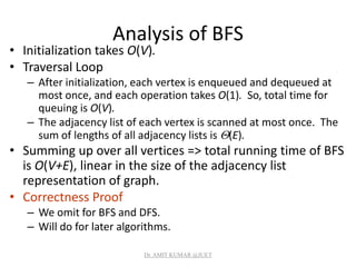
45. Analysis of DFS
• Loops on lines 1-2 & 5-7 take (V) time, excluding time
to execute DFS-Visit.
• DFS-Visit is called once for each white vertex vV when
it’s painted gray the first time. Lines 3-6 of DFS-Visit is
executed |Adj[v]| times. The total cost of executing
DFS-Visit is vV|Adj[v]| = (E)
• Total running time of DFS is (V+E).
Dr. AMIT KUMAR @JUET

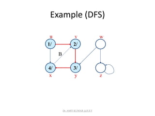
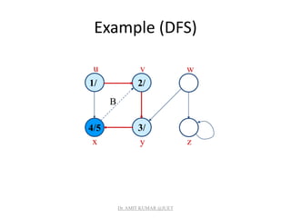
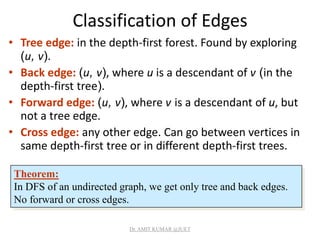
46. Depth-First Trees
• Predecessor subgraph defined slightly different from
that of BFS.
• The predecessor subgraph of DFS is G = (V, E) where
E ={([v],v) : v  V and [v]  NIL}.
– How does it differ from that of BFS?
– The predecessor subgraph G forms a depth-first forest
composed of several depth-first trees. The edges in E are
called tree edges.
Definition:
Forest: An acyclic graph G that may be disconnected.
Dr. AMIT KUMAR @JUET

47. Classification of Edges
• Tree edge: in the depth-first forest. Found by exploring
(u, v).
• Back edge: (u, v), where u is a descendant of v (in the
depth-first tree).
• Forward edge: (u, v), where v is a descendant of u, but
not a tree edge.
• Cross edge: any other edge. Can go between vertices in
same depth-first tree or in different depth-first trees.
Theorem:
In DFS of an undirected graph, we get only tree and back edges.
No forward or cross edges.
Dr. AMIT KUMAR @JUET