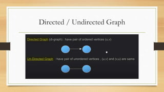
This document discusses graphs and graph algorithms. It defines graphs as consisting of nodes and edges. It describes two common representations of graphs: adjacency matrices and adjacency lists. It then explains several graph algorithms, including breadth-first search, depth-first search, minimum spanning tree algorithms like Prim's and Kruskal's, and shortest path algorithms like Dijkstra's and Floyd-Warshall.

1. GRAPHS
ALGORITHMS
By Ashwin Shiv
NIT Delhi

2. GRAPHS
• A Graph is a non-linear data structure consisting of nodes and edges.
• The nodes are sometimes also referred to as vertices
• edges are lines or arcs that connect any two nodes in the graph.
• undirected graph
• weighted graphs

3. Directed / Undirected Graph

4. Common Representations of Graphs
• 1. Adjacency Matrix
• 2. Adjacency List

5. Adjacency Matrix
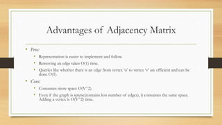
• Adjacency Matrix is a 2D array of size V x V where V is the number of
vertices in a graph.
• Let the 2D array be adj[][], a slot adj[i][j] = 1 indicates that there is an edge
from vertex i to vertex j.
• Adjacency matrix for undirected graph is always symmetric.
• Adjacency Matrix is also used to represent weighted graphs. If adj[i][j] = w,
then there is an edge from vertex i to vertex j with weight w.

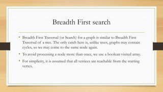
6. Representation of Adjacency Matrix
Matrix[][]

7. Advantages of Adjacency Matrix
• Pros:
• Representation is easier to implement and follow.
• Removing an edge takes O(1) time.
• Queries like whether there is an edge from vertex ‘u’ to vertex ‘v’ are efficient and can be
done O(1).
• Cons:
• Consumes more space O(V^2).
• Even if the graph is sparse(contains less number of edges), it consumes the same space.
Adding a vertex is O(V^2) time.

8. Adjacency List
• An array of lists is used.
• Size of the array is equal to the number of vertices.
• Let the array be array[]. An entry array[i] represents the list of vertices
adjacent to the ith vertex.
• This representation can also be used to represent a weighted graph.
• The weights of edges can be represented as lists of pairs. Following is
adjacency list representation of the above graph.

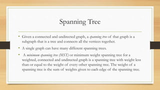
9. Representation of Adjacency List
array[] of List

10. Advantages of Adjacency List
• Pros:
• Saves space O(|V|+|E|) .
• In the worst case, there can be C(V, 2) number of edges in a graph thus consuming O(V^2)
space.
• Adding a vertex is easier.
• Cons:
• Queries like whether there is an edge from vertex u to vertex v are not efficient and can be
done O(V).

11. Graphs Implemenations
• Elementary Graph Algorithms ( MATRIX / ARRAY)
• Breadth First search ( QUEUE)
• Depth First search ( STACK )
• Minimum Spanning Tree :
• Prim’s Minimum Spanning Tree
• Kruskal’s Minimum Spanning Tree Algorithm
• Shortest Paths :
• Dijkstra Algorithm (Single-source shortest path )
• Floyd-Warshall algorithm ( all Pair Shortest Path )

12. Breadth First search
• Breadth First Traversal (or Search) for a graph is similar to Breadth First
Traversal of a tree. The only catch here is, unlike trees, graphs may contain
cycles, so we may come to the same node again.
• To avoid processing a node more than once, we use a boolean visited array.
• For simplicity, it is assumed that all vertices are reachable from the starting
vertex.

13. Depth First search
• Depth First Traversal (or Search) for a graph is similar to Depth First
Traversal of a tree.
• The only catch here is, unlike trees, graphs may contain cycles, so we may
come to the same node again.
• To avoid processing a node more than once, we use a boolean visited array.

14. Spanning Tree
• Given a connected and undirected graph, a spanning tree of that graph is a
subgraph that is a tree and connects all the vertices together.
• A single graph can have many different spanning trees.
• A minimum spanning tree (MST) or minimum weight spanning tree for a
weighted, connected and undirected graph is a spanning tree with weight less
than or equal to the weight of every other spanning tree. The weight of a
spanning tree is the sum of weights given to each edge of the spanning tree.

15. Kruskal’s Minimum Spanning Tree Algorithm
Algorithm
• Sort all the edges in non-decreasing order of their weight.
• Pick the smallest edge. Check if it forms a cycle with the spanning tree formed so far. If
cycle is not formed, include this edge. Else, discard it.
• Repeat step#2 until there are (V-1) edges in the spanning tree.

16. Prim’s Minimum Spanning Tree
• Algorithm
1) Create a set mstSet that keeps track of vertices already included in MST.
2) Assign a key value to all vertices in the input graph. Initialize all key values as
INFINITE. Assign key value as 0 for the first vertex so that it is picked first.
3) While mstSet doesn’t include all vertice
• Pick a vertex u which is not there in mstSet and has minimum key value
• Include u to mstSet.
• Update key value of all adjacent vertices of u. To update the key values, iterate through all
adjacent vertices. For every adjacent vertex v, if weight of edge u-v is less than the previous
key value of v, update the key value as weight of u-v

17. Dijkstra Algorithm (Single-source shortest path )
• Dijkstra’s algorithm, We maintain two sets, one set contains vertices included in shortest path tree, other set includes
vertices not yet included in shortest path tree. At every step of the algorithm, we find a vertex which is in the other set (set
of not yet included) and has a minimum distance from the source.
• Below are the detailed steps used in Dijkstra’s algorithm to find the shortest path from a single source vertex to all other
vertices in the given graph.
Algorithm
1) Create a set sptSet (shortest path tree set) that keeps track of vertices included in shortest path tree, i.e., whose minimum
distance from source is calculated and finalized. Initially, this set is empty.
2) Assign a distance value to all vertices in the input graph. Initialize all distance values as INFINITE. Assign distance value
as 0 for the source vertex so that it is picked first.
3) While sptSet doesn’t include all vertices
a) Pick a vertex u which is not there in sptSet and has minimum distance value.
b) Include u to sptSet.
c) Update distance value of all adjacent vertices of u. To update the distance values, iterate through , is less than the
distance value of v, then update the distance value of v.

18. Floyd-Warshall algorithm ( All Pair Shortest Path )
• The Floyd Warshall Algorithm is for solving the All Pairs Shortest Path problem.
• The problem is to find shortest distances between every pair of vertices in a given
edge weighted directed Graph.
• We initialize the solution matrix same as the input graph matrix as a first step
• Then we update the solution matrix by considering all vertices as an intermediate
vertex.
• The idea is to one by one pick all vertices and updates all shortest paths which
include the picked vertex as an intermediate vertex in the shortest path.

19. References:
• geeksforgeeks.org
• Youtube channel by Abdul Bari
(https://www.youtube.com/channel/UCZCFT11CWBi3MHNlGf019nw)