Downloaded 106 times


![Expectations for Continuous
Random Variables
The mean of X, denoted μX , is defined as the
expected value of X
The variance of X, denoted σX
2 , is defined as the
expectation of the squared deviation, (X - μX)2, of a
random variable from its mean
Copyright © 2010 Pearson Education, Inc. Publishing as Prentice Hall
E(X)μX
])μE[(Xσ 2
X
2
X
Ch. 5-15
5.2](https://image.slidesharecdn.com/chap05continuousrandomvariablesandprobabilitydistributions-191217014943/85/Chap05-continuous-random-variables-and-probability-distributions-15-320.jpg)


![Covariance
Let X and Y be continuous random variables, with
means μx and μy
The expected value of (X - μx)(Y - μy) is called the
covariance between X and Y
An alternative but equivalent expression is
If the random variables X and Y are independent, then the
covariance between them is 0. However, the converse is not true.
Copyright © 2010 Pearson Education, Inc. Publishing as Prentice Hall
)]μ)(YμE[(XY)Cov(X, yx
yxμμE(XY)Y)Cov(X,
Ch. 5-60](https://image.slidesharecdn.com/chap05continuousrandomvariablesandprobabilitydistributions-191217014943/85/Chap05-continuous-random-variables-and-probability-distributions-60-320.jpg)

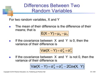
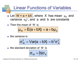
![Linear Combinations of
Random Variables
A linear combination of two random variables, X and Y,
(where a and b are constants) is
The mean of W is
Copyright © 2010 Pearson Education, Inc. Publishing as Prentice Hall
bYaXW
YXW bμaμbY]E[aXE[W]μ
Ch. 5-65](https://image.slidesharecdn.com/chap05continuousrandomvariablesandprobabilitydistributions-191217014943/85/Chap05-continuous-random-variables-and-probability-distributions-65-320.jpg)

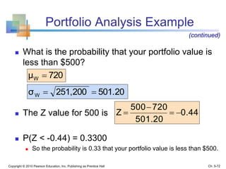

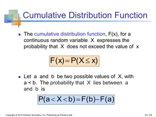
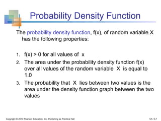
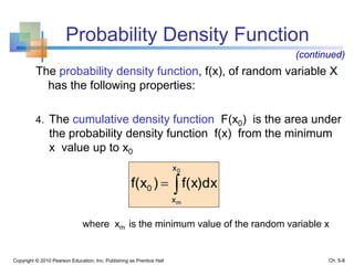
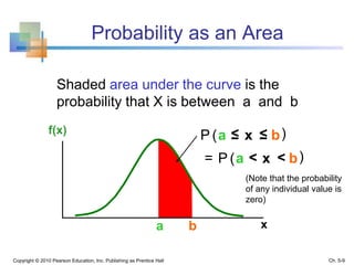
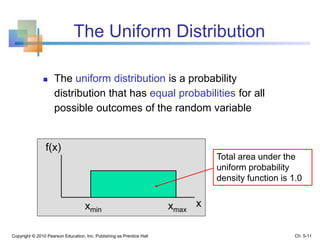
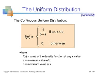
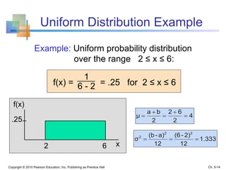
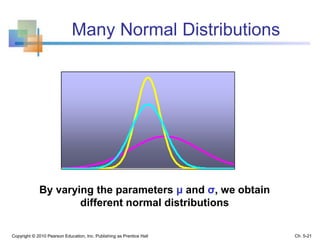
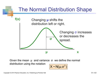
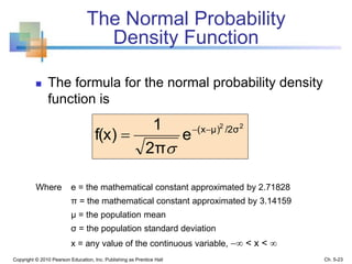
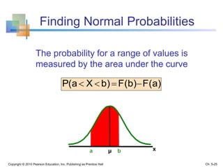
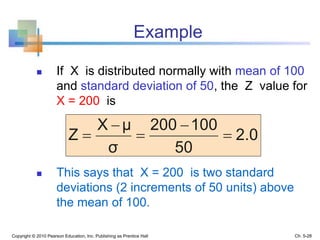
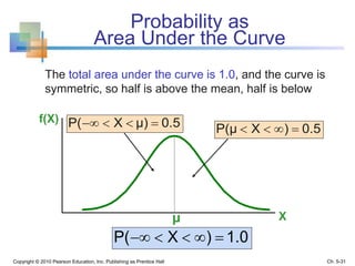
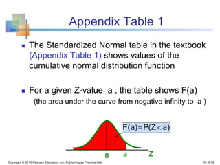
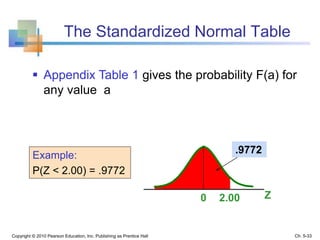
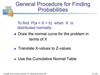
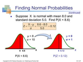
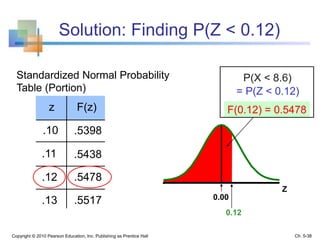
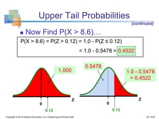
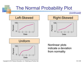
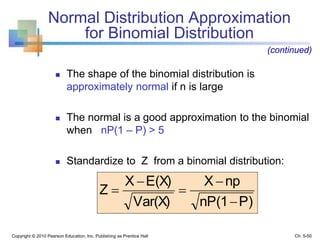
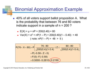
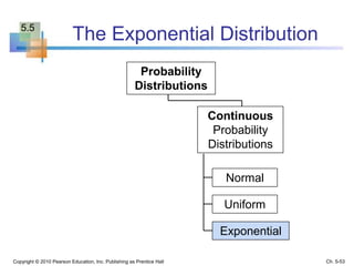
This chapter discusses continuous random variables and probability distributions, including the normal distribution. It introduces continuous random variables and their probability density functions. It describes the key characteristics and properties of the uniform and normal distributions. It also discusses how to calculate probabilities using the normal distribution, including how to standardize a normal distribution and use normal distribution tables.


