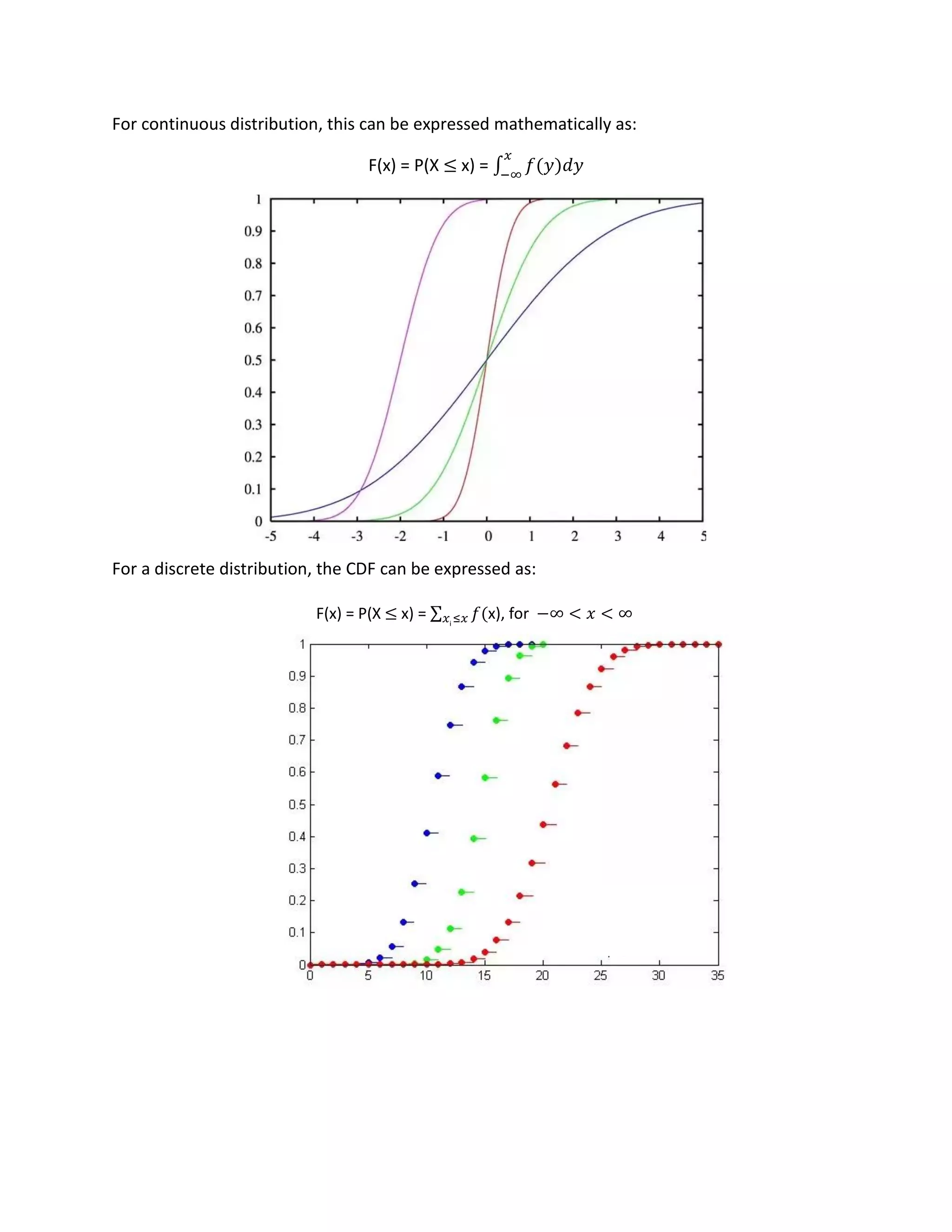
The document discusses cumulative distribution functions (CDFs) and probability density functions (PDFs) for continuous random variables. It provides definitions and properties of CDFs and PDFs. For CDFs, it describes how they give the probability that a random variable is less than or equal to a value. For PDFs, it explains how they provide the probability of a random variable taking on a particular value. The document also gives examples of CDFs and PDFs for exponential and uniform random variables.

1. Cumulative Distributive Function (CDF) :-
Intuition behind CDF:
Several of the most important concepts introduced in the study of discrete distributions
also play an important role for continuous distributions.
Let X be a discrete random variable that takes on values from the set.
{0,
1
𝑁
,
2
𝑁
, … … … … … ,
𝑁 − 1
𝑁
}
With equal probability that is:
PX(
𝐾
𝑁
) =
1
𝑁
𝑓𝑜𝑟 𝑘 = 0,1,2, … … , (𝑁 − 1)
Such type of random variables are generated in high level languages such as FORTRAN, C,
and MATLAB. In such cases, N is taken to be very large. So that random variable can fall anywhere
in interval (0, 1). Consider N∞, so that Random variable can fall anywhere in the interval [0, 1).
We see that:
PX(
𝐾
𝑁
) =
1
𝑁
=
1
∞
= 0
i.e. each point has a zero probability of occurring (Yet something has to occur). Now, it is
clear that Probability Mass Function (PMF) cannot be used for continuous random variable.
Hence, we need alternative description for continuous random variable. Since a continuous
random variable will typically has a zero probability to occur, events of the form {𝑋 ≤ 𝑥} can be
considered.
It is sometimes useful to provide cumulative probabilities. Such probabilities can be used
to find the probability mass function of a random variable. Therefore, using cumulative
probabilities is an alternate method of describing the probability distribution of a random
variable.
Definition:
“The cumulative distribution function (CDF), P(X ≤ x) or F(X), is the probability that the
variable(X) takes a value less than or equal to some specific x.”
The cumulative distribution function (CDF) calculates the cumulative probability for a
given x-value. Use the CDF to determine the probability that a random observation that is taken
from the population will be less than or equal to a certain value. You can also use this information
to determine the probability that an observation will be greater than a certain value, or between
two values.

2. For continuous distribution, this can be expressed mathematically as:
F(x) = P(X ≤ x) = ∫ 𝑓(𝑦)𝑑𝑦
𝑥
−∞
For a discrete distribution, the CDF can be expressed as:
F(x) = P(X ≤ x) = 𝑓(𝑥 ≤𝑥 x), for −∞ < 𝑥 < ∞i

3. Exponential random variable:
The cumulative distribution function is given by
Proof:
For x ≥ 0:
FX(x) = Pr{X ≤ 𝑥} = fX(y) dy
FX(x) = ∫
1
𝑏
𝑥
−∞
exp (−
𝑥
𝑏
) u(y) dy
FX(x) = ∫
1
𝑏
𝑥
0
e-(y/b) dy
FX(x) =
1
𝑏
[(e-(y/b))/(-1/b)]0
𝑥
FX(x) = -e-(y/b)
FX(x) = 1 – exp(−
𝑥
𝑏
) ux
For x < 0:
FX(x) = 0
Properties:
1)
a. FX(−∞) = Pr{ X ≤ −∞ } = 0
b. FX(+∞) = Pr{ X ≤ +∞ } = 1
Proof:
By definition, FX (a) = P(A) where A = {X ≤ a}. Then F(= +∞) = P(A), with A = {X ≤ +∞}. This
event is the certain event, since A = {X ≤ +∞} = {X ∈ R} = S (S for Sample Space). Therefore
F(= +∞) = P(S) = 1. Similarly, Then F(= −∞) = P(A), with A = {X ≤ −∞}. This event is the
impossible event, random variable X is a real variable, so F(= −∞) = P(∅) = 0.
2) Since CDF is a probability so it must take on values between ‘0’ and ‘1’.
0 ≤ FX(x) ≤ 1
∫
∞
−∞

4. Proof:
As minimum FX(−∞) = Pr{ X ≤ −∞ } = 0 and maximum FX(+∞) = Pr{ X ≤ +∞ } = 1. So
FX(x) should be lie between [0, 1].
3) For fixed x1 and x2 if x1 ≤ x2 then FX(x1) ≤ FX(x2).
Consider tub events {X ≤ x1} and {X ≤ x2}, then the former is the subset of the later. (i.e. if the
former event occurs, we must be in the later as well.)
If x1 < x2 then FX(x) = Pr{X ≤ 𝑥}
This implies that CDF is a Monotonic Non-Decreasing Function. (It will never decrease in
any case.)
Proof:
This is a consequence of the fact that probability is a non-decreasing function, i.e. if
A ⊆ B then P(A) ≤ P(B). Indeed, recall that if A ⊆ B then the set B can be partitioned into
B = A + (B ∩ A), so, using the additivity property of probability, P(B) = P(A) + P(B ∩ A) ≥ P(A).
If x1 ≤ x2, then the corresponding events A = {X ≤ x1} and B = {X ≤ x2} have the property that
A ⊂ B. Therefore P{X ≤ x1} _ P{X ≤ x2}, which by the definition of a CDF means F(x1) ≤ F(x2).
4) For x1 < x2
Pr{x1 < X ≤ 𝑥2} = FX(x2) - FX(x1)
Proof:
Consider {X ≤ 𝑥2}, we can break it into two mutually exclusive events.
(−∞, 𝑥2] = (−∞, 𝑥1] ∪ (𝑥1, 𝑥2]
Pr{X ≤ 𝑥2} = {X ≤ 𝑥1} ∪ {x1 < X ≤ 𝑥2}
Pr{X ≤ 𝑥2} = Pr{X ≤ 𝑥1} + Pr{x1 < X ≤ 𝑥2}
FX(x2) = FX(x1) + Pr{x1 < X ≤ 𝑥2}
Pr{x1 < X ≤ 𝑥2} = FX(x2) - FX(x1)
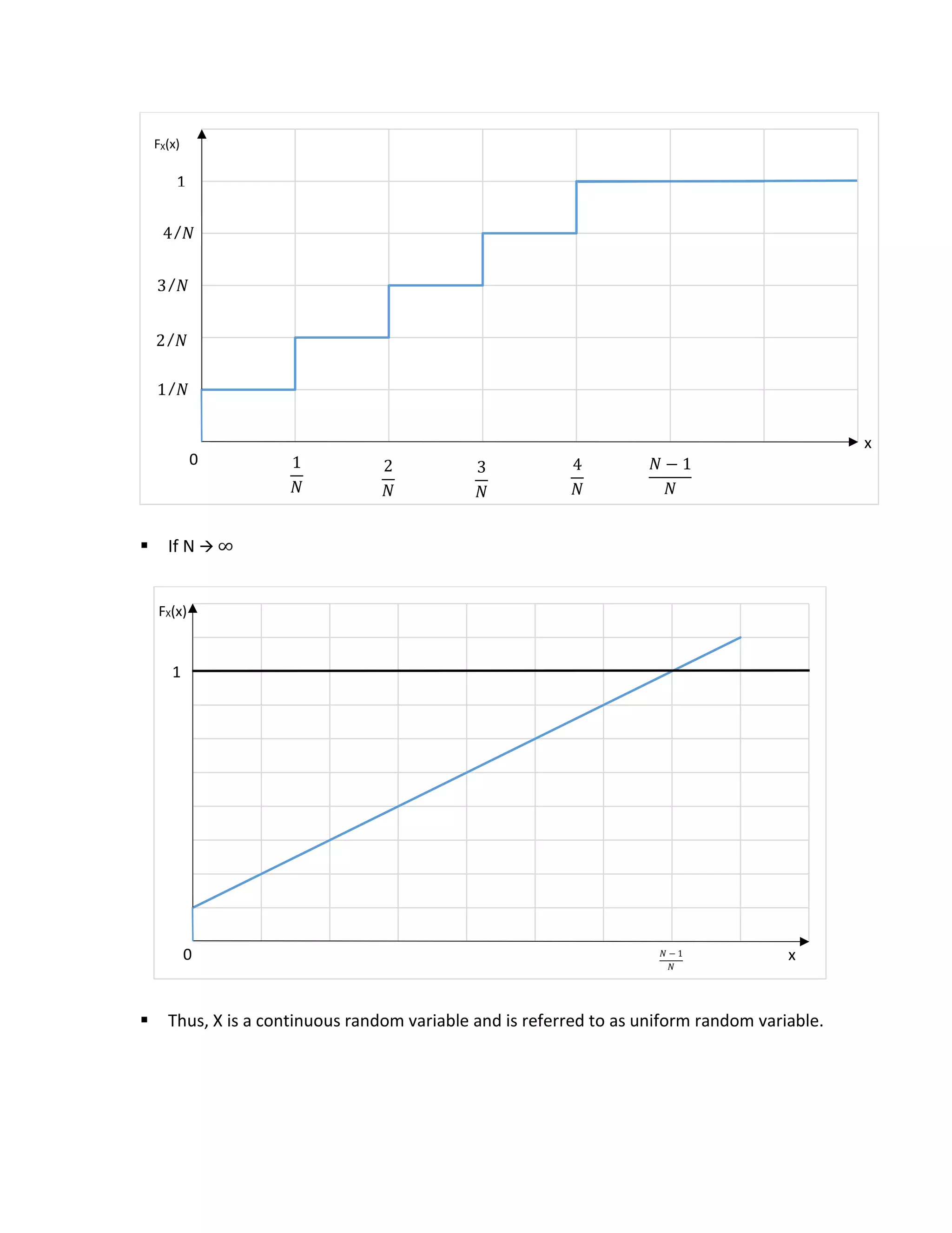
Note:
 If x<0 then FX(x) = 0
 If x ≥
𝑁−1
𝑁
then FX(x) = 1
 If 0 < k < N ∀ 𝑥 ∈ [
𝑘−1
𝑁
,
𝑘
𝑁
)  FX(x) =
𝑘
𝑁

5.  If N  ∞
 Thus, X is a continuous random variable and is referred to as uniform random variable.
0
1
1
4 𝑁
3 𝑁
2 𝑁
1 𝑁
1
𝑁
2
𝑁
3
𝑁
4
𝑁
𝑁 − 1
𝑁
FX(x)
x
FX(x)
x𝑁 − 1
𝑁
0

6. Probability Density Function (PDF):
Intuition behind PDF:
It is often difficult to work with CDF i.e. for a Gaussian random variable, one of the most
commonly used random variable. Its CDF does not exist in closed form. An alternative
description is often used. Defined as:
fX(x) = lim
∈→0
𝑃(𝑥≤𝑋<(𝑥+∈))
∈
If a variable is continuous, between any two possible values of the variable are an infinite
number of other possible values, even though we cannot distinguish some of them from one
another in practice. It is therefore not possible to count the number of possible values of a
continuous variable. In this situation calculus provides the logical means of finding probabilities.
Definition:
The probability of X lying in an infinities many small interval around x, normalize by the
length of the interval. That’s why it called density.
The probability density function helps identify regions of higher and lower probabilities
for values of a random variable.
For continuous random variable:
The probability density function (PDF) is an equation that represents the probability
distribution of a continuous random variable.
In the above bar chart of cork diameters, each bar represents the percent of corks with
that corresponding diameter.
r

7. General Expression:
Pr(𝑥 ≤ 𝑋 < (𝑥+∈)) = FX(x + ∈) - FX(x)
fX(x) = lim
∈→0
𝑃(𝑥≤𝑋<(𝑥+∈))
∈
fX(x) = lim
∈→0
F (x + ∈) − F (x)
∈
fx(x) =
𝑑
𝑑𝑥
FX(x)
FX(x) = fx(x) dx
Hence PDF of a random variable X is the derivative of CDF. CDF is the area under the curve.
FX(x) = Pr{X ≤ 𝑥} = fx(y) dy
For discrete random variable:
Experiments where there is more than one outcome, each having a possibly different
probability. The probability density function of a discrete random variable is simply the
collection of all these probabilities.
The discrete probability density function (PDF) of a discrete random variable X can be
represented in a table, graph, or formula, and provides the probabilities Pr(X = x) for all possible
values of x.
This bar chart displays the PDF for candy color. Each bar represents the probability of candies of
that color expressed as a percentage.
r
X X
∫
∫
𝑥
−∞

8. For exponential random variable:
An exponential random variable has a PDF of the form
fX(x) =
where 𝜆 is a positive parameter characterizing the PDF. This is a legitimate PDF because
fx(x) dx = 𝜆𝑒 dx = −𝑒 0
∞
= 1
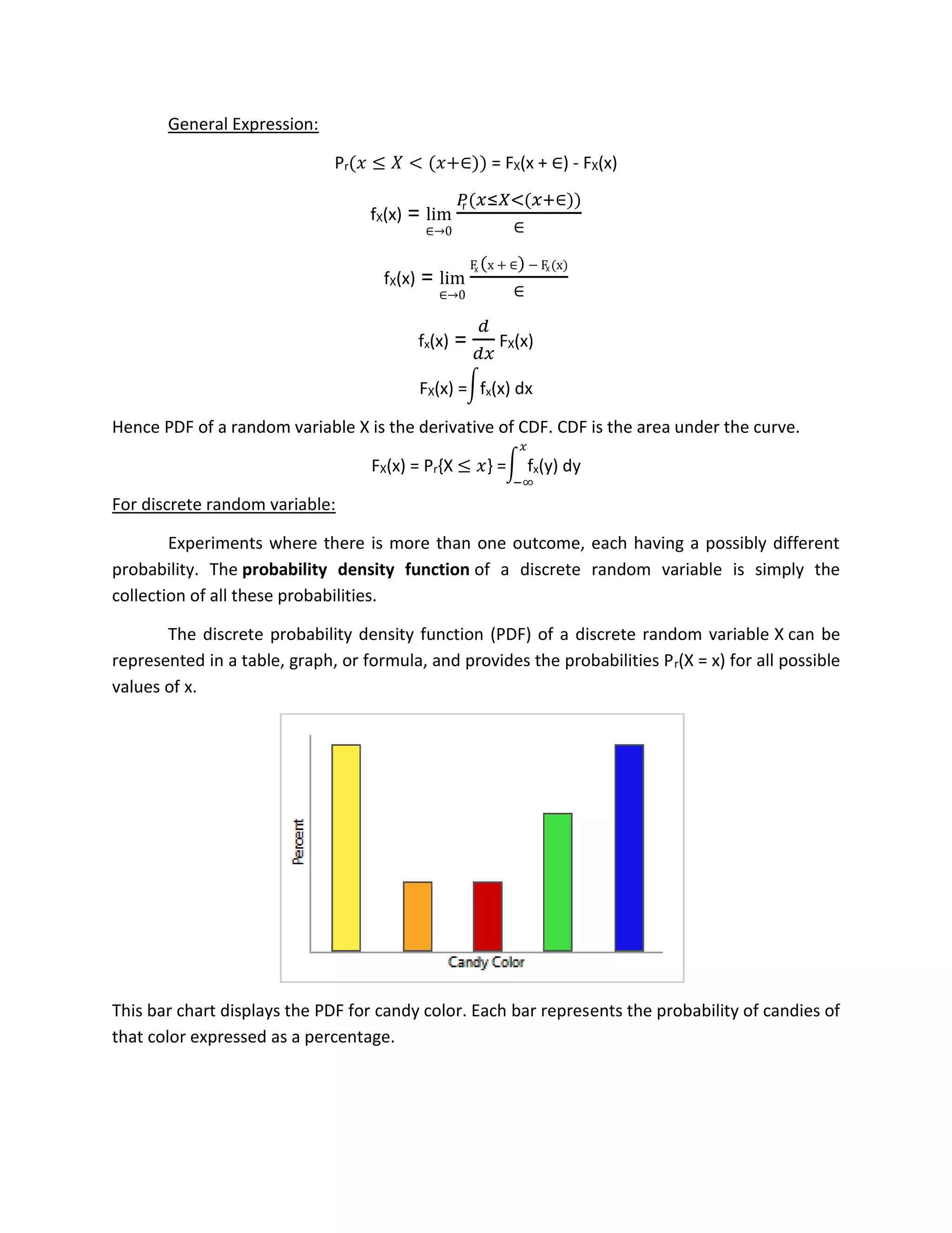
Properties of PDF:
1) fx(x) ≥ 0 for all values of x since F is non-decreasing.
2) fx(x) =
𝑑
𝑑𝑥
FX(x)
3) FX(x) = Pr{X ≤ 𝑥} = fx(y) dy
4) fx(x) dx = 1
5) fX(x) = Pr(𝑎 ≤ 𝑋 ≤ 𝑏)
6) lim
𝑥→−∞
𝑓(𝑥) = 0 = lim
𝑥→∞
𝑓(𝑥)
7) *In the continuous case P(X = c) = 0 for every possible value of c.
8) *This has a very useful consequence in the continuous case:
Pr (a ≤ X ≤ b) = Pr (a < X ≤ b) = Pr (a ≤ X < b) = Pr (a < X < b)
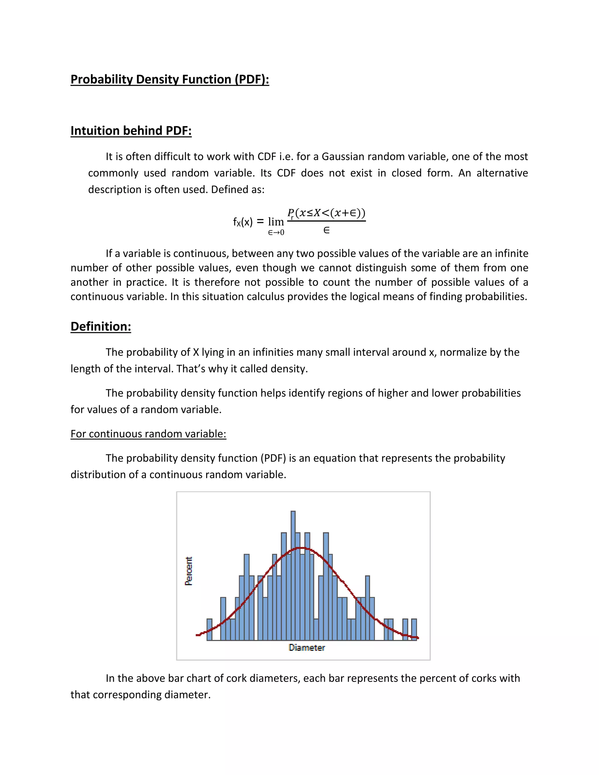
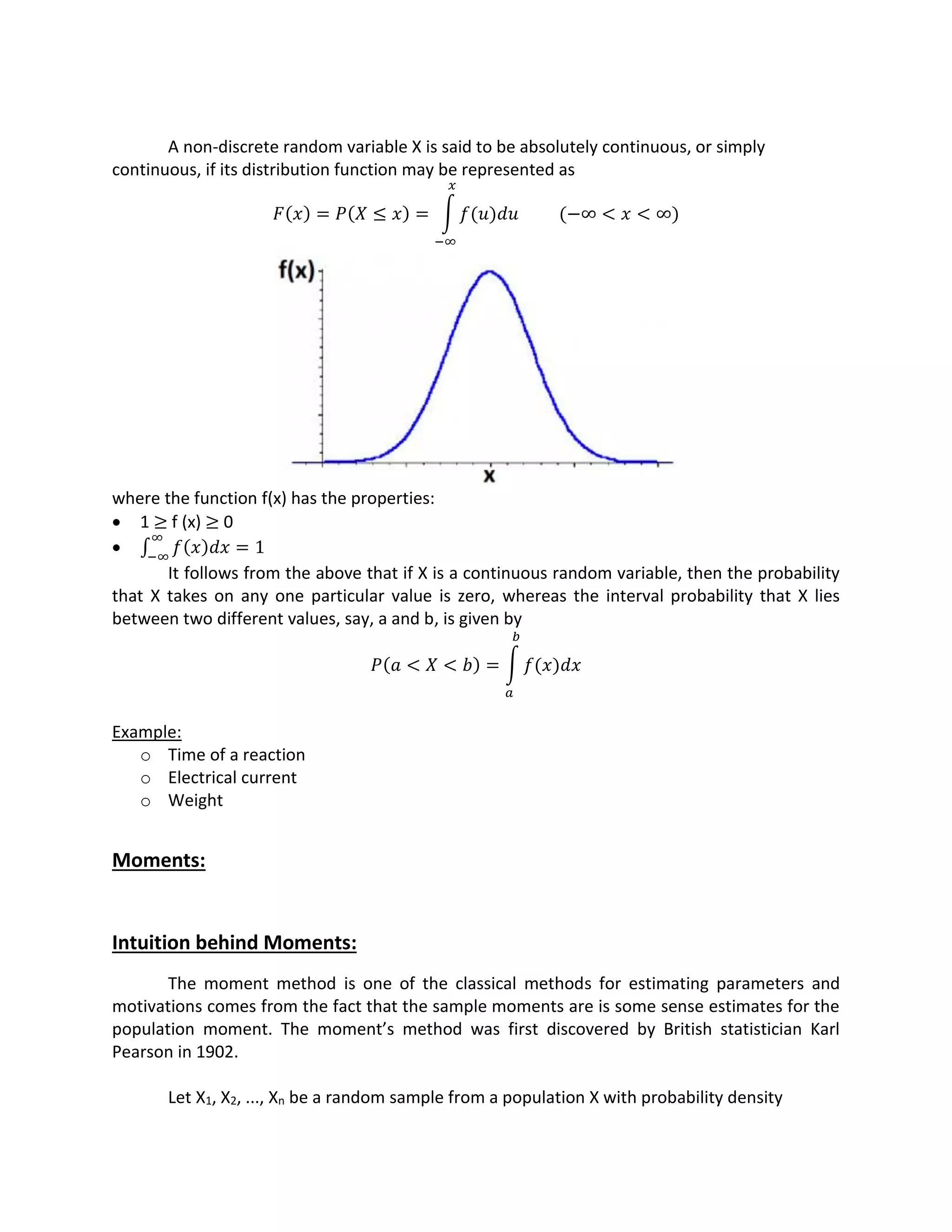
Continuous Random Variable:
A continuous random variable is a random variable with an interval (either finite or
infinite) of real numbers for its range.
Random variables that can assume any one of the uncountable infinite numbers of
points in one or more intervals on the real line are called continuous random variables. If a
random variable X assumes every possible value in an interval [a, b] or (−∞,+∞) is called
continuous random variable.
A continuous distribution describes the probabilities of the possible values of a
continuous random variable. A continuous random variable is a random variable with a set of
possible values (known as the range) that is infinite and uncountable.
Probabilities of continuous random variables (X) are defined as the area under the curve
of its PDF. Thus, only ranges of values can have a nonzero probability. The probability that a
continuous random variable equals some value is always zero.
∫
𝑥
−∞
∫
∞
−∞
∫
𝑏
𝑎
𝜆𝑒 if x ≥ 0−𝜆𝑥
0 otherwise
∫
∞
−∞
−𝜆𝑥 −𝜆𝑥
∫
∞
0

9. A non-discrete random variable X is said to be absolutely continuous, or simply
continuous, if its distribution function may be represented as
𝐹(𝑥) = 𝑃(𝑋 ≤ 𝑥) = ∫ 𝑓(𝑢)𝑑𝑢
𝑥
−∞
(−∞ < 𝑥 < ∞)
where the function f(x) has the properties:
 1 ≥ f (x) ≥ 0
 ∫ 𝑓(𝑥)𝑑𝑥 = 1
∞
−∞
It follows from the above that if X is a continuous random variable, then the probability
that X takes on any one particular value is zero, whereas the interval probability that X lies
between two different values, say, a and b, is given by
𝑃(𝑎 < 𝑋 < 𝑏) = ∫ 𝑓(𝑥)𝑑𝑥
𝑏
𝑎
Example:
o Time of a reaction
o Electrical current
o Weight
Moments:
Intuition behind Moments:
The moment method is one of the classical methods for estimating parameters and
motivations comes from the fact that the sample moments are is some sense estimates for the
population moment. The moment’s method was first discovered by British statistician Karl
Pearson in 1902.
Let X1, X2, ..., Xn be a random sample from a population X with probability density

10. function f(x; θ1, θ2, ..., θm), where θ1, θ2, ..., θm are m unknown parameters. Let
be the kth population moment about 0. Further, let
be the kth moment about zero.
In moment method, we find the estimator for the parameters θ1, θ2, ..., θm by equating
the first m population moments (if they exist) to the first m sample moments, that is
E (X) = M1
E(X2) = M2
E(X3) = M3
.
.
.
E (Xm) = Mm
The moment-generating function of a random variable is an alternative specification of
its probability distribution. Thus, it provides the basis of an alternative route to analytical results
compared with working directly with probability density functions or cumulative distribution
functions. There are particularly simple results for the moment-generating functions of
distributions defined by the weighted sums of random variables. Note, however, that not all
random variables have moment-generating functions.
In addition to univariate distributions, moment-generating functions can be defined for
vector- or matrix-valued random variables, and can even be extended to more general cases.
The moment-generating function does not always exist even for real-valued arguments,
unlike the characteristic function. There are relations between the behavior of the moment-
generating function of a distribution and properties of the distribution, such as the existence of
moments.

11. Definition:
The nth moment of a random variable X is define as:
E(xn) = xn fX(x) dx
E(xn) = xk
n PX (xk)
E(x2) = x2 fX(x) dx
𝛾 =
(𝑥 − 𝑥̅)
𝑥 − 1
𝛾 = √
(𝑥 − 𝑥̅)
𝑥 − 1
𝛾2 = E [(x - 𝜇x)2]
𝛾2 = E [(x2 + 𝜇x2 – 2x 𝜇x]
𝛾2 = E (x2) + 𝜇x2 – 2E(x) 𝜇x
𝛾2 = E (x2) + 𝜇x2 – 2𝜇x 𝜇x
𝛾2 = E (x2) + 𝜇x2 – 2𝜇x2
𝛾2 = E (x2) - 𝜇x2
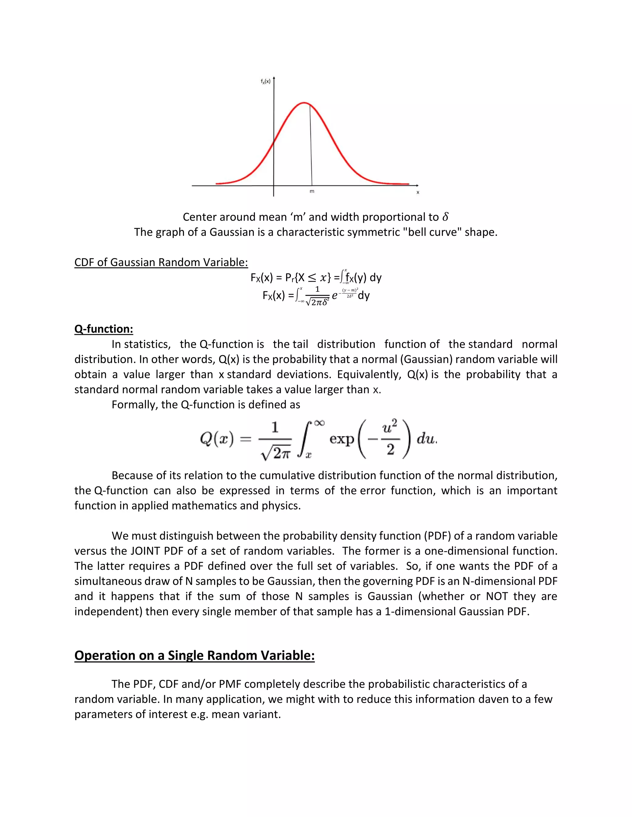
Gaussian Random Variables:
One of the most important random variable since many physical phenomena can be
modeled as Gaussian random variable e.g. thermal noise in electronic components, students
grading etc. It is named after the mathematician Carl Friedrich Gauss.
The PDF is:
fX(x) =
1
√2𝜋𝛿
𝑒
Its PDF has two parameters:
Mean = m
𝛿 = Standard Derivation
𝛿2 = Variance
Gaussian functions are often used to represent the probability density function of a normally
distributed random variable.
Shortened Notation:
X ~ N (m, 𝛾2)
∫
∞
−∞
∑
𝑘
∫
∞
−∞
2
2
2
i
2
−
(𝑥 − 𝑚)
2𝛿
2
2

12. Center around mean ‘m’ and width proportional to 𝛿
The graph of a Gaussian is a characteristic symmetric "bell curve" shape.
CDF of Gaussian Random Variable:
FX(x) = Pr{X ≤ 𝑥} = fX(y) dy
FX(x) =
1
√2𝜋𝛿
𝑒 dy
Q-function:
In statistics, the Q-function is the tail distribution function of the standard normal
distribution. In other words, Q(x) is the probability that a normal (Gaussian) random variable will
obtain a value larger than x standard deviations. Equivalently, Q(x) is the probability that a
standard normal random variable takes a value larger than x.
Formally, the Q-function is defined as
Because of its relation to the cumulative distribution function of the normal distribution,
the Q-function can also be expressed in terms of the error function, which is an important
function in applied mathematics and physics.
We must distinguish between the probability density function (PDF) of a random variable
versus the JOINT PDF of a set of random variables. The former is a one-dimensional function.
The latter requires a PDF defined over the full set of variables. So, if one wants the PDF of a
simultaneous draw of N samples to be Gaussian, then the governing PDF is an N-dimensional PDF
and it happens that if the sum of those N samples is Gaussian (whether or NOT they are
independent) then every single member of that sample has a 1-dimensional Gaussian PDF.
Operation on a Single Random Variable:
The PDF, CDF and/or PMF completely describe the probabilistic characteristics of a
random variable. In many application, we might with to reduce this information daven to a few
parameters of interest e.g. mean variant.
∫
𝑥
−∞
2
2−
(𝑦 − 𝑚)
2𝛿∫
𝑥
−∞
2

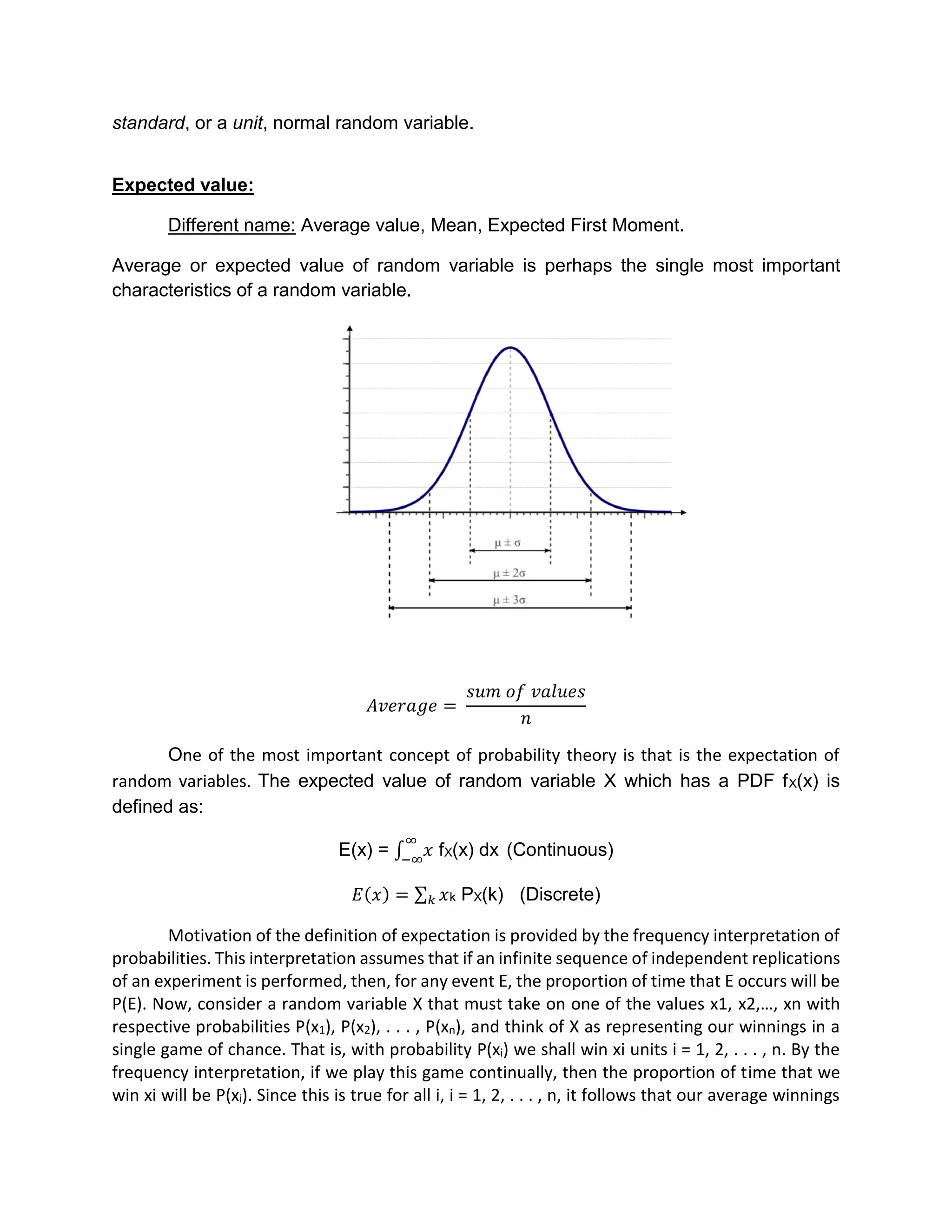
13. Expected value of function of random variable:
The concept of expectation can be applied to function of random variables as well. If X is
continuous, then the expectation of g(X) is defined as,
E[g(x)] = ∫ 𝑔(𝑥)
∞
−∞
fX(x) dx (Continuous Random Variable)
where f is the probability density function of X.
If X is discrete, then the expectation of g(X) is defined as, then,
E[g(x)) = 𝑔𝑘 (xk)PX(k) (Discrete Random Variable)
where f is the probability mass function of X and X is the support of X.
If E(X) = −∞ or E(X) = ∞ (i.e., E(|X|) = ∞), then we say the expectation E(X) does not
exist. The expectation operator has inherits its properties from those of summation and
integral.
For example if X is original Random variable, you might be interested in what happen to
the mean if you scale by
Y = cx
Normal Random Variables:
We say that X is a normal random variable, or simply that is normally distributed,
with parameters 𝜇 and 𝛿2. If the density of X is given by:
The normal random variables was introduced by the French mathematician
Abraham de Moivre in 1733, who used it to approximate associated with binomial
random variables when the binomial parameter n is large. The result was later extended
by Laplace and other and is now encompassed in a probability theorem known as the
central limit theorem. The central limit theorem, one of the two most important result in
the probability theory gives a theoretical base to the often noted empirical observation
that, in practice, in example many random phenomena abbey, at least approximately, a
normal probability distribution. Some example of random phenomena obeying this
behavior are the height of a man, the velocity in any direction of a molecule in gas, and
the error made in the measuring a physical quantity.
An important implication of the preceding result is that if X is normally distributed
with parameters 𝜇 and 𝛿2, then
𝑍 =
(𝑥 − 𝜇)
𝛿
is normally distributed with parameters 0 and 1. Such a random variable is said to be a

14. standard, or a unit, normal random variable.
Expected value:
Different name: Average value, Mean, Expected First Moment.
Average or expected value of random variable is perhaps the single most important
characteristics of a random variable.
𝐴𝑣𝑒𝑟𝑎𝑔𝑒 =
𝑠𝑢𝑚 𝑜𝑓 𝑣𝑎𝑙𝑢𝑒𝑠
𝑛
One of the most important concept of probability theory is that is the expectation of
random variables. The expected value of random variable X which has a PDF fX(x) is
defined as:
E(x) = ∫ 𝑥
∞
−∞
fX(x) dx (Continuous)
𝐸(𝑥) = 𝑥𝑘 k PX(k) (Discrete)
Motivation of the definition of expectation is provided by the frequency interpretation of
probabilities. This interpretation assumes that if an infinite sequence of independent replications
of an experiment is performed, then, for any event E, the proportion of time that E occurs will be
P(E). Now, consider a random variable X that must take on one of the values x1, x2,…, xn with
respective probabilities P(x1), P(x2), . . . , P(xn), and think of X as representing our winnings in a
single game of chance. That is, with probability P(xi) we shall win xi units i = 1, 2, . . . , n. By the
frequency interpretation, if we play this game continually, then the proportion of time that we
win xi will be P(xi). Since this is true for all i, i = 1, 2, . . . , n, it follows that our average winnings

15. per game will be:
𝑥𝑛
𝑖=1 i P(xi) = E[X]
The probability concept of expectation is analogous to the physical concept of
center of gravity of distribution of mass.
Exponential random variable:
In probability theory and statistics, the exponential distribution (also known as negative
exponential distribution) is the probability distribution that describes the time between events
in a Poisson point process, i.e., a process in which events occur continuously and independently
at a constant average rate. It is a particular case of the gamma distribution. It is the continuous
analogue of the geometric distribution, and it has the key property of being memoryless. In
addition to being used for the analysis of Poisson point processes it is found in various other
contexts.
The exponential distribution is not the same as the class of exponential families of
distributions, which is a large class of probability distributions that includes the exponential
distribution as one of its members, but also includes the normal distribution, binomial
distribution, gamma distribution, Poisson, and many others.
Exponential random variable can be defined as:
fX(x) =
1
𝑏
exp (−
𝑥
𝑏
) u(x)
E(x) = ∫ 𝑥
∞
−∞
fX(x) dx
E(x) = ∫ 𝑥
∞
−∞
1
𝑏
exp (−
𝑥
𝑏
) u(x) dx
E(x) = ∫ 𝑥
∞
0
1
𝑏
e (-x/b) d(x)
Let y=
𝑥
𝑏
limits: y =
0
𝑏
= 0; y =
∞
𝑏
= ∞
dy =
1
𝑏
dx dx = b dy
E(x) = b ∫ 𝑦
∞
0
e-y dy
Integration by parts:
E(x) = b [y (e-y/-1) – ∫(𝑒-y/-1) dy]0
∞
E(x) = b [-y e-y + ∫ 𝑒-y dy]0
∞

16. E(x) = b [-y e-y - e-y ]0
∞
∎ lim
𝑦→∞
𝑒-y = 0
E(x) = b[0 – (0-1)]
E(x) = b
The exponential distribution often arises as the distribution of the amount of time
until some specific event occurs. For instance, the amount of time until an earth quake
occurs, or until a new war breaks out, or until a telephone call you receive turns out to be
a wrong number are all random variables that tend in practice to have exponential
distributions.
An exponential random variable can be a very good model for the amount of time
until a piece of equipment breaks down, until a light bulb burns out, or until an accident
occur.
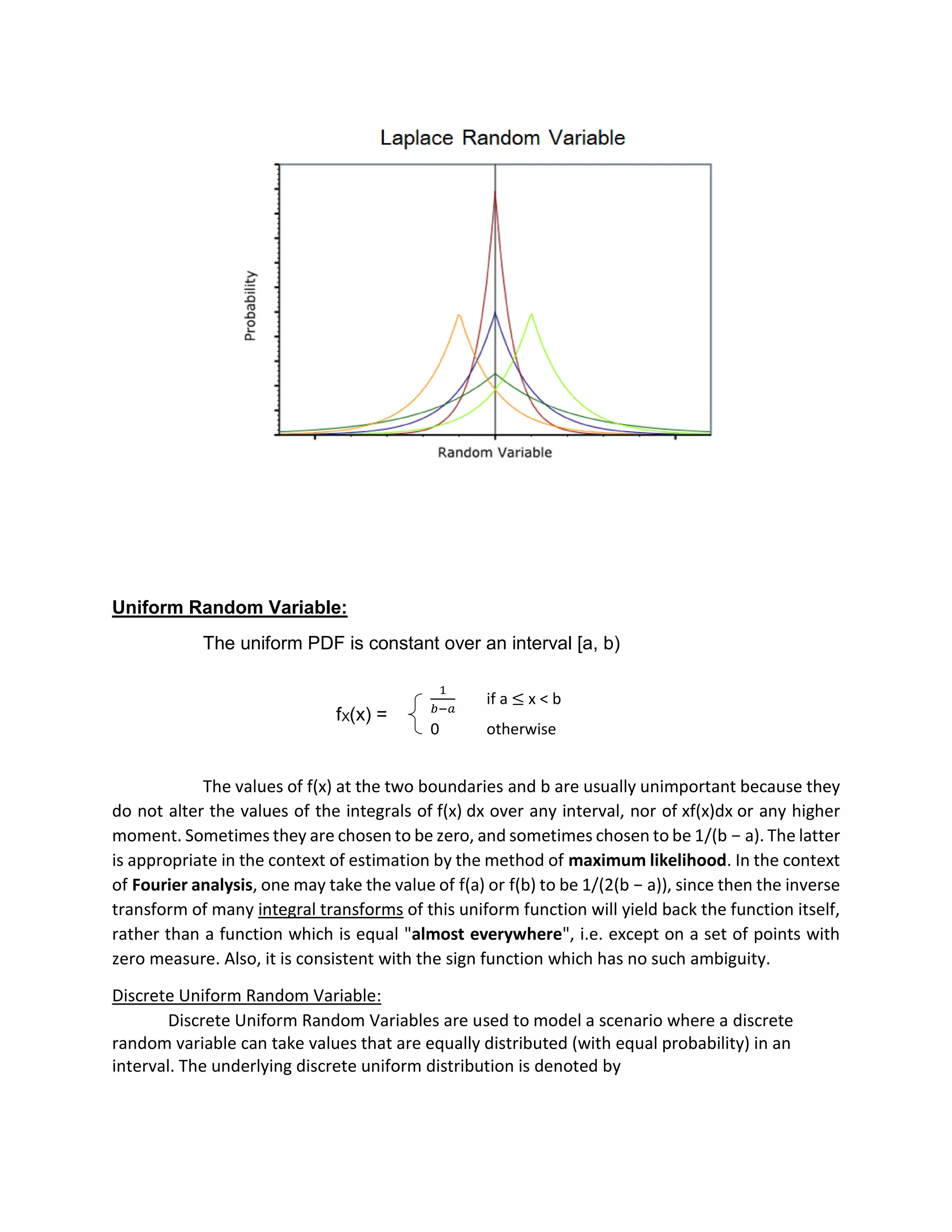
Laplacian Random Variable:
In probability theory and statistics, the Laplace distribution is a continuous probability
distribution named after Pierre-Simon Laplace. It is also sometimes called the double
exponential distribution, because it can be thought of as two exponential distributions (with an
additional location parameter) spliced together back-to-back, although the term is also
sometimes used to refer to the Gumbel distribution. The difference between two independent
identically distributed exponential random variables is governed by a Laplace distribution, as is
a Brownian motion evaluated at an exponentially distributed random time. Increments
of Laplace motion or a variance gamma process evaluated over the time scale also have a Laplace
distribution.
FX(x) =
1
2𝑏
exp (−
|𝑥|
𝑏
)

17. Uniform Random Variable:
The uniform PDF is constant over an interval [a, b)
fX(x) =
The values of f(x) at the two boundaries and b are usually unimportant because they
do not alter the values of the integrals of f(x) dx over any interval, nor of xf(x)dx or any higher
moment. Sometimes they are chosen to be zero, and sometimes chosen to be 1/(b − a). The latter
is appropriate in the context of estimation by the method of maximum likelihood. In the context
of Fourier analysis, one may take the value of f(a) or f(b) to be 1/(2(b − a)), since then the inverse
transform of many integral transforms of this uniform function will yield back the function itself,
rather than a function which is equal "almost everywhere", i.e. except on a set of points with
zero measure. Also, it is consistent with the sign function which has no such ambiguity.
Discrete Uniform Random Variable:
Discrete Uniform Random Variables are used to model a scenario where a discrete
random variable can take values that are equally distributed (with equal probability) in an
interval. The underlying discrete uniform distribution is denoted by
1
𝑏−𝑎
if a ≤ x < b
0 otherwise

18. X∼U(S)
Where S is a finite set of discrete points on the real line. Meaning that each element in the
finite set are equally likely.
There are many applications in which it is useful to run simulation experiments.
Many programming languages have the ability to generate pseudo-random numbers which are
effectively distributed according to the standard uniform distribution.