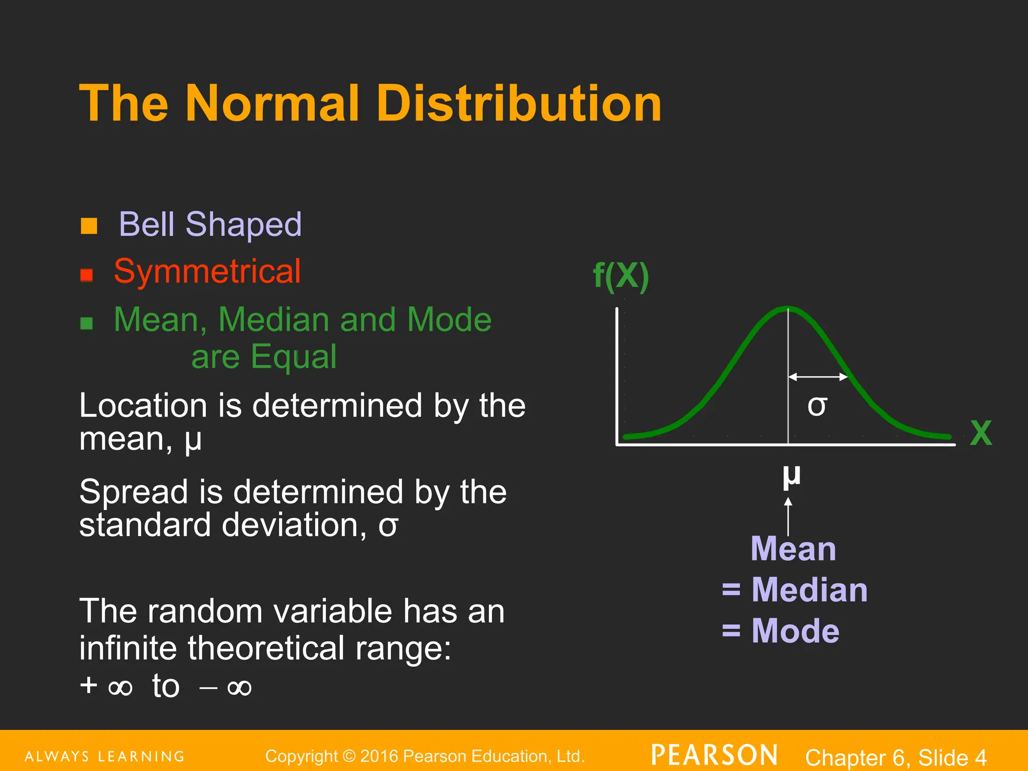
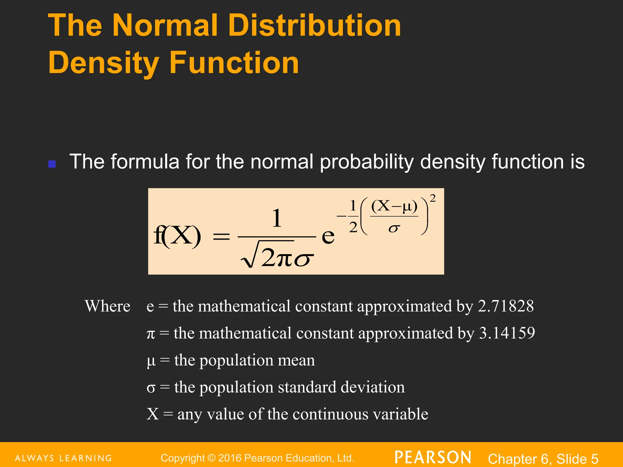
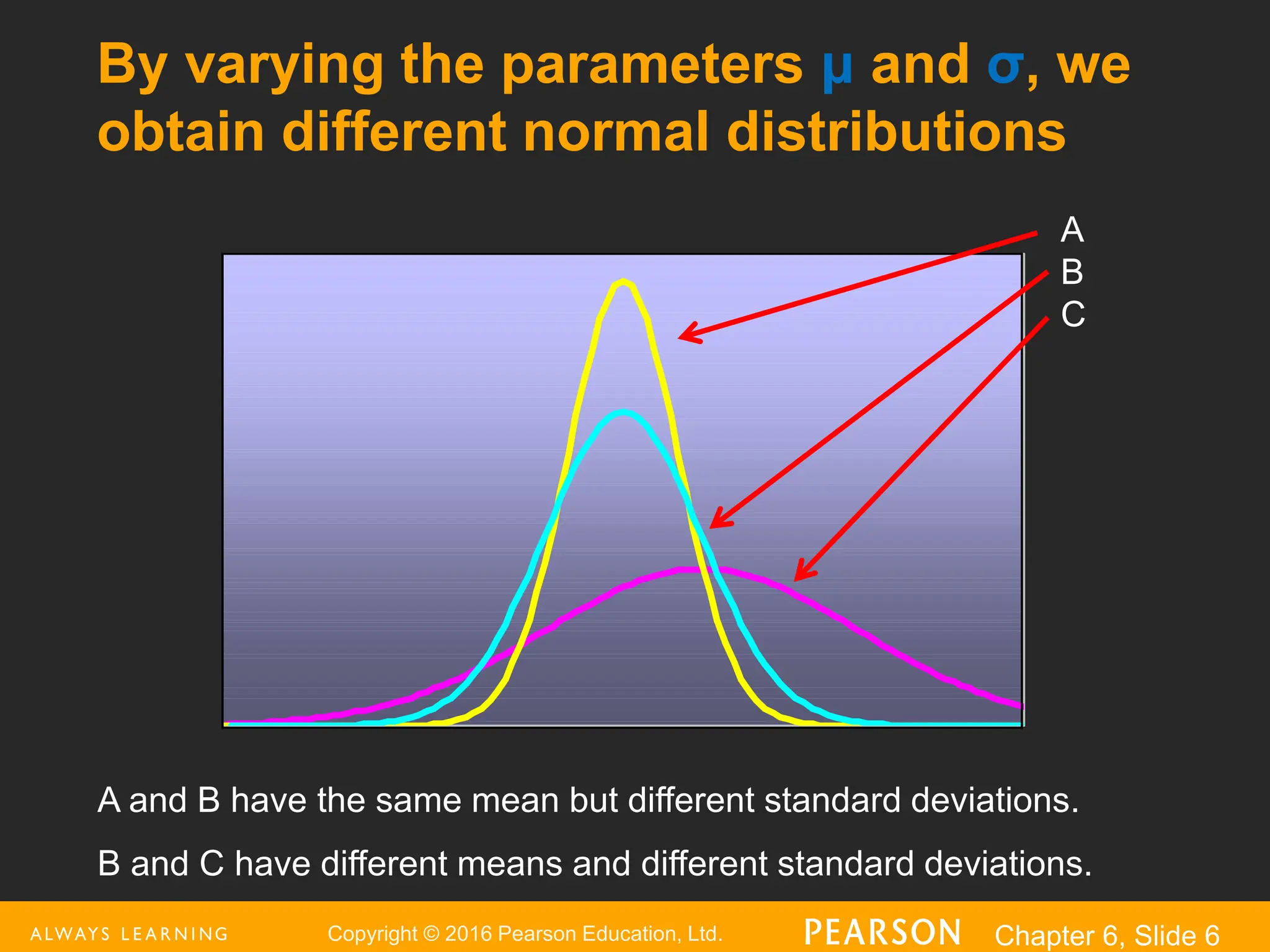
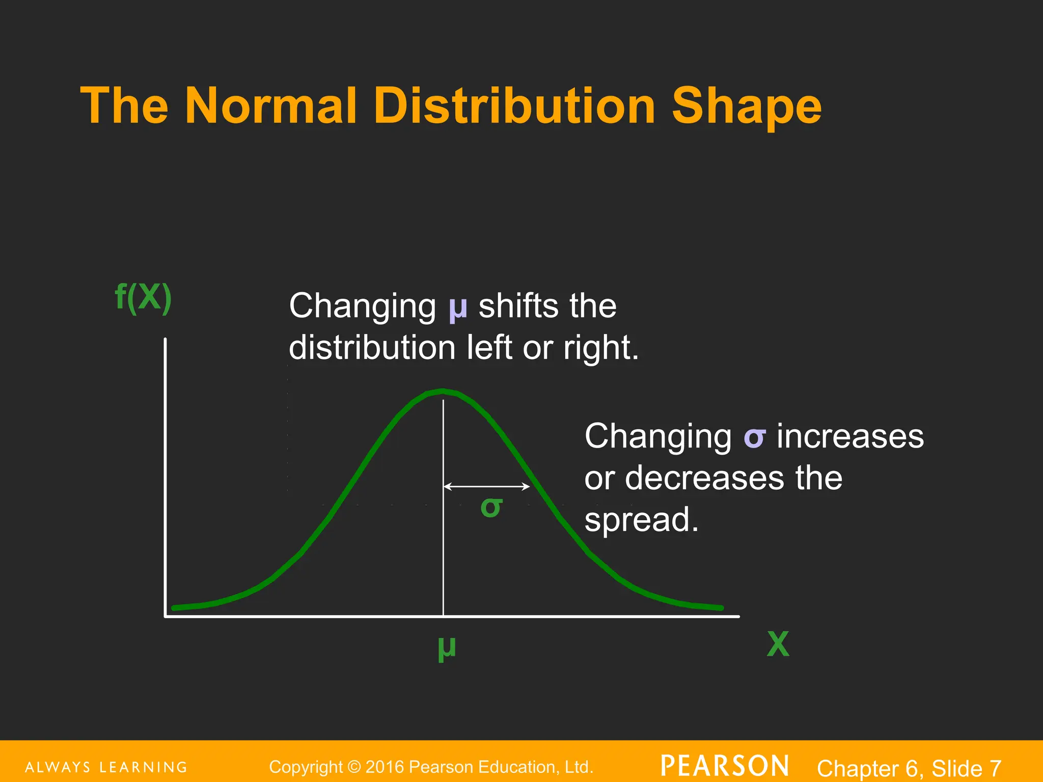
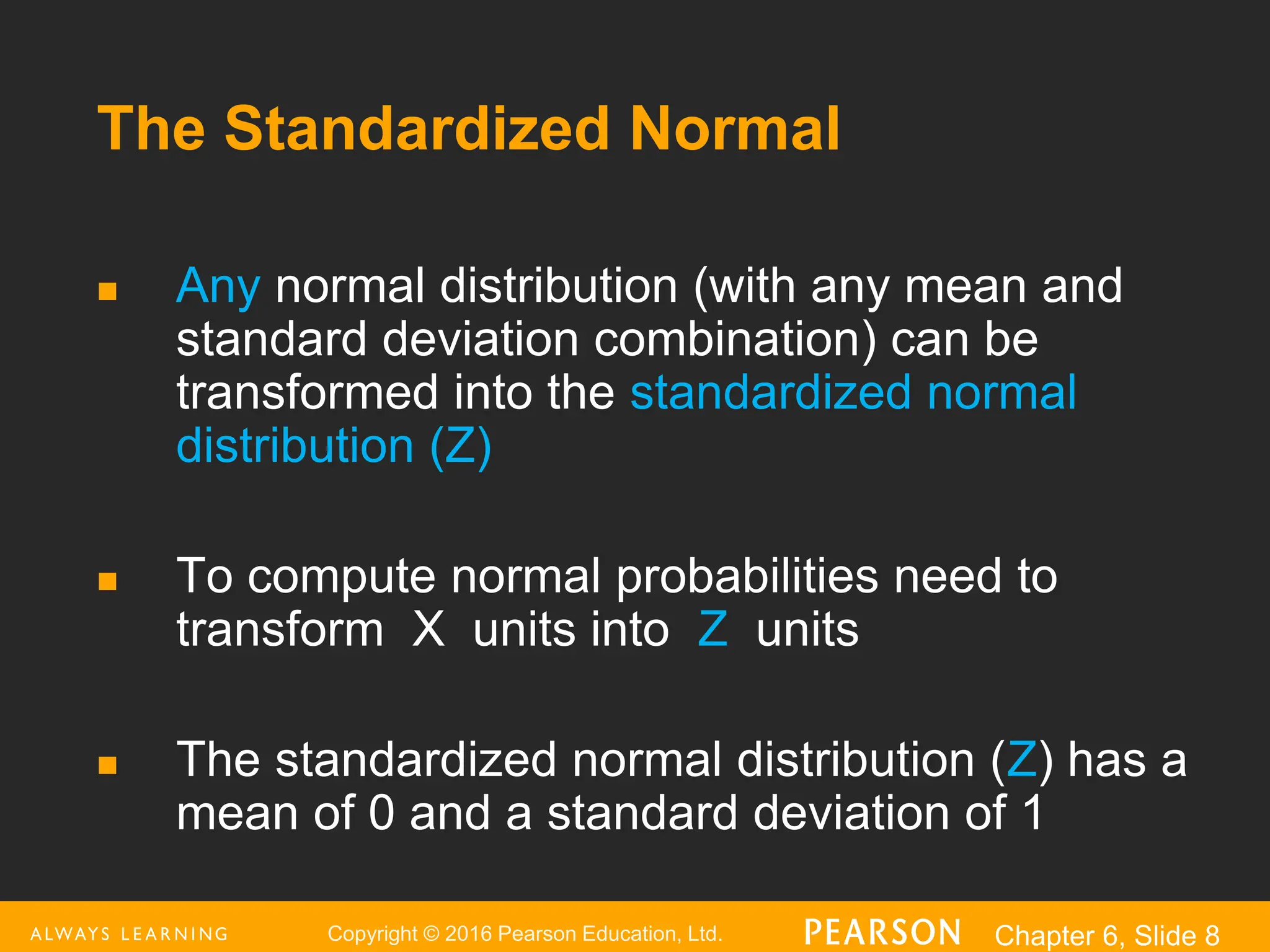
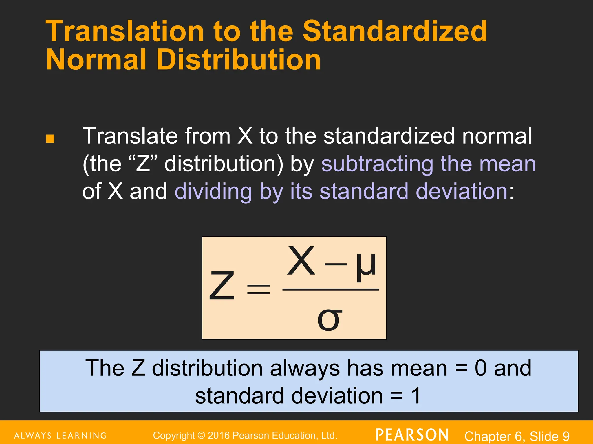
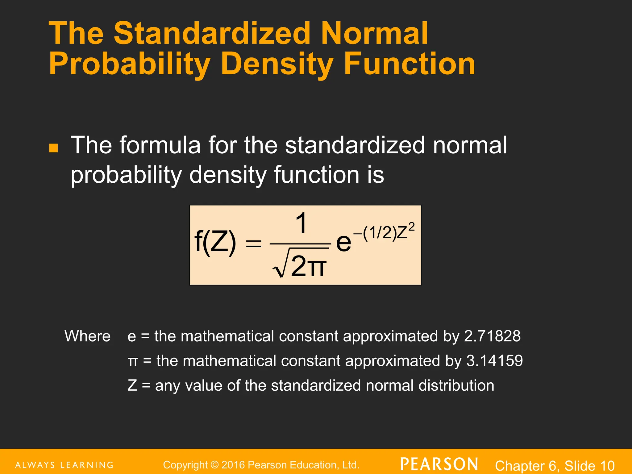
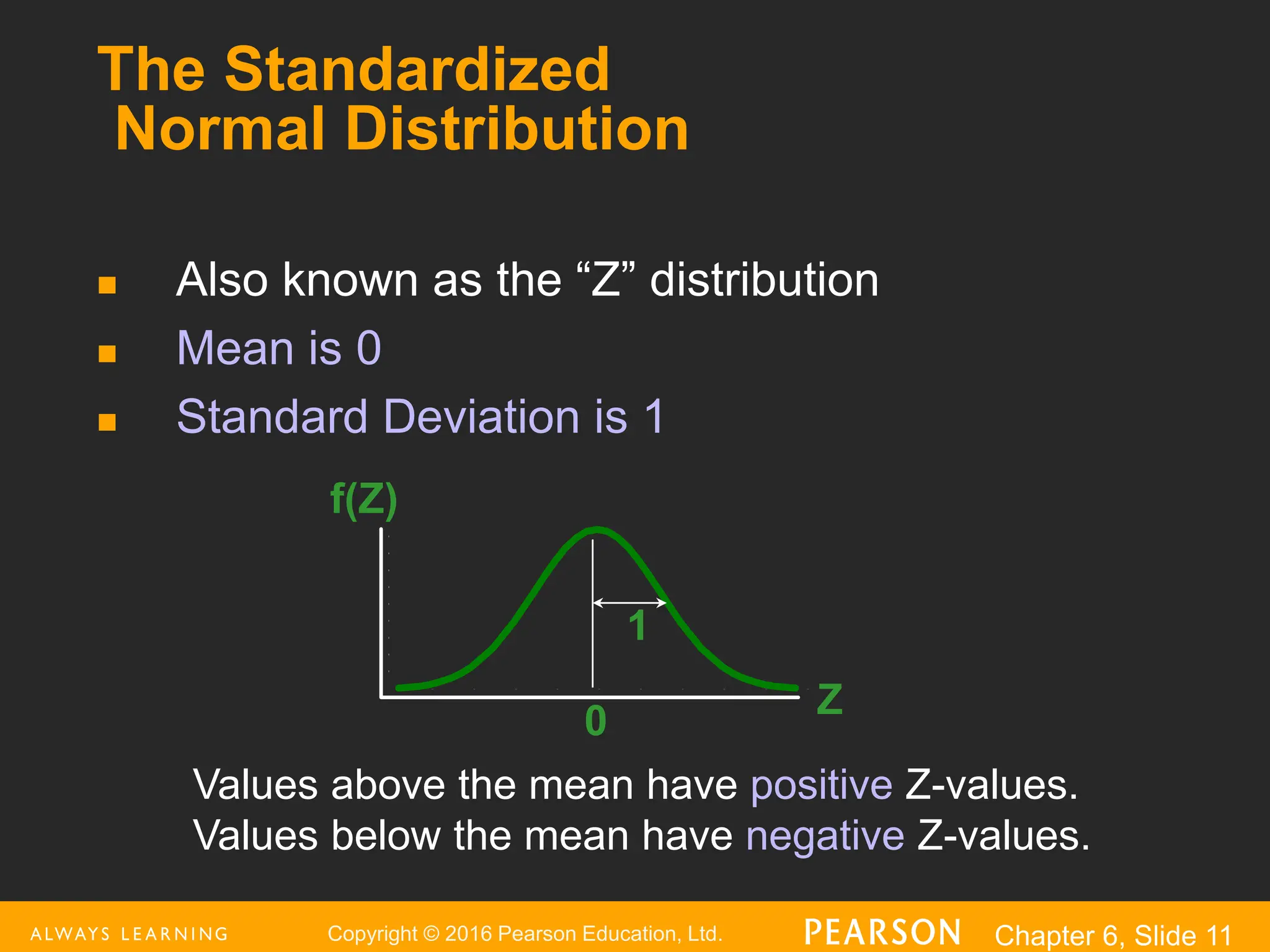
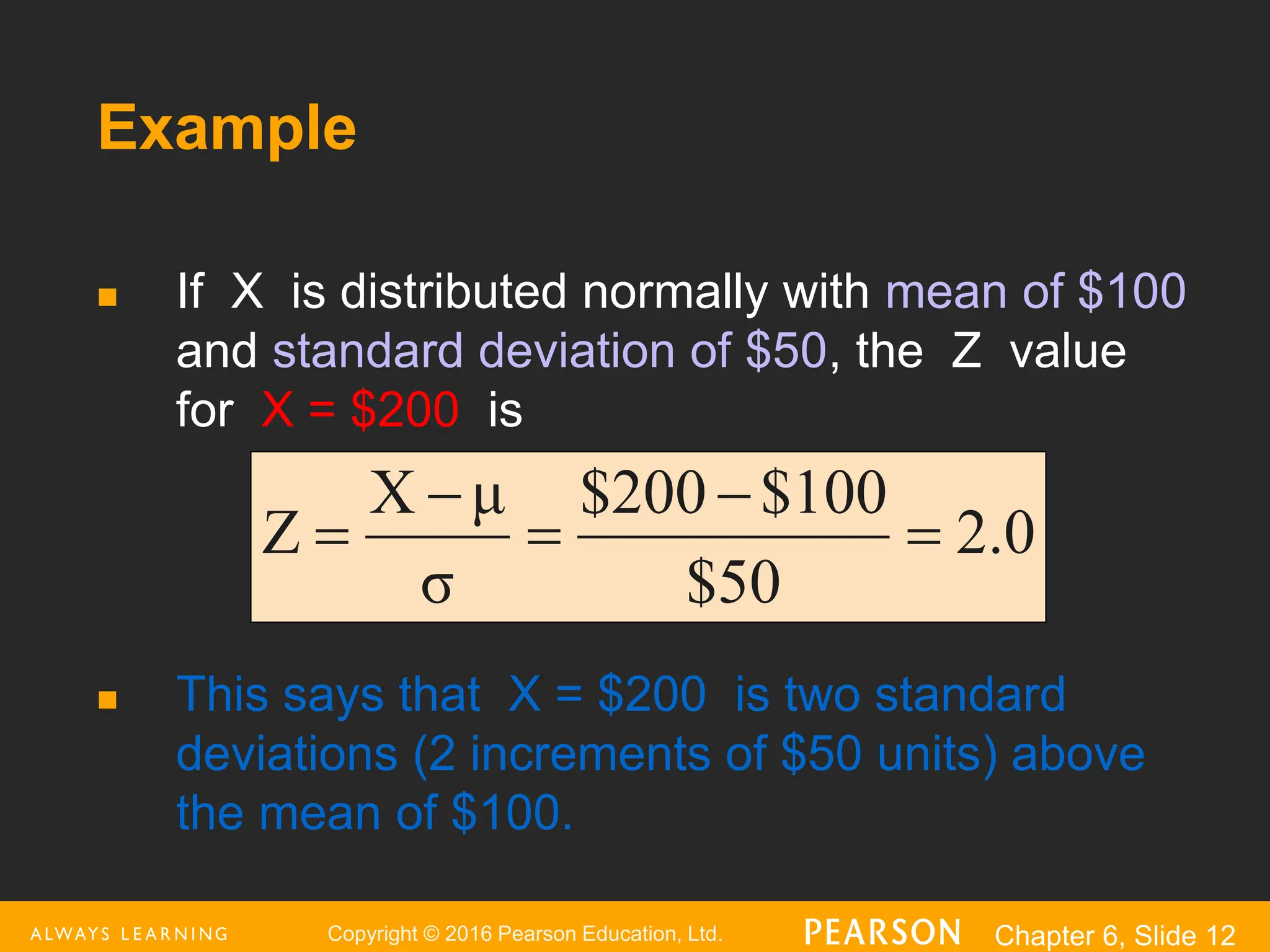
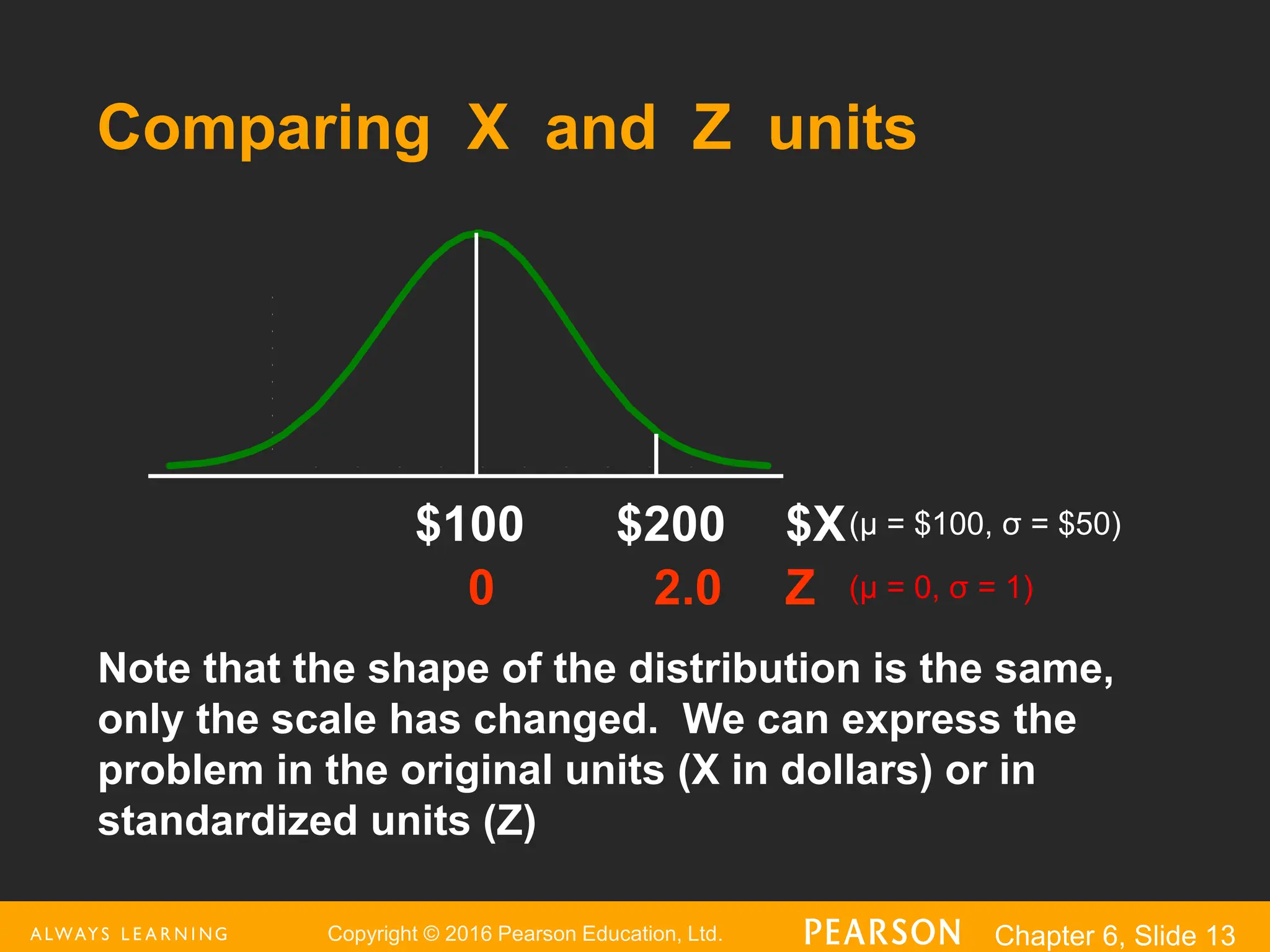
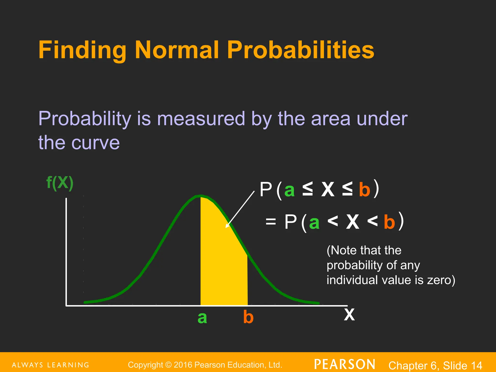
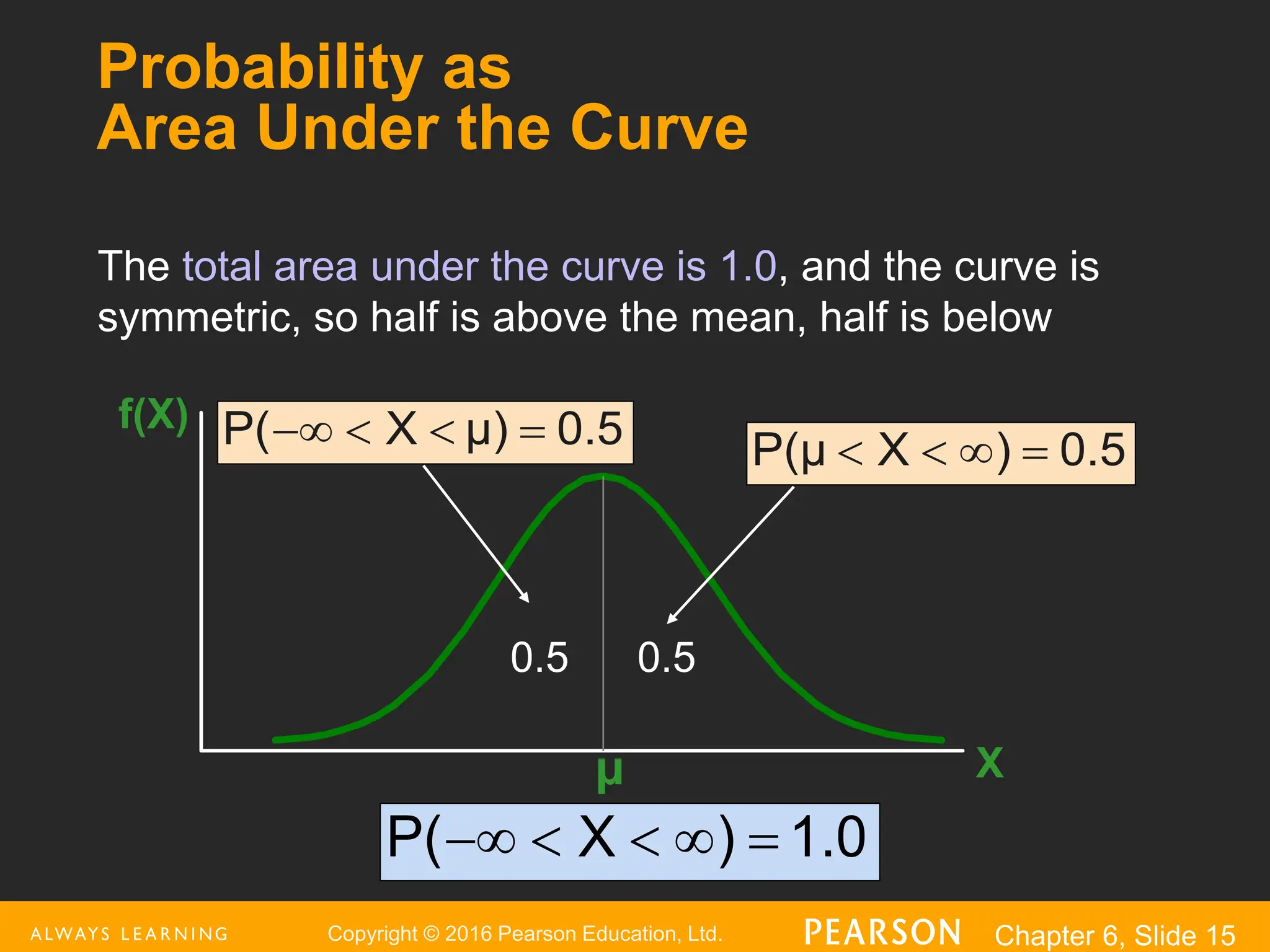
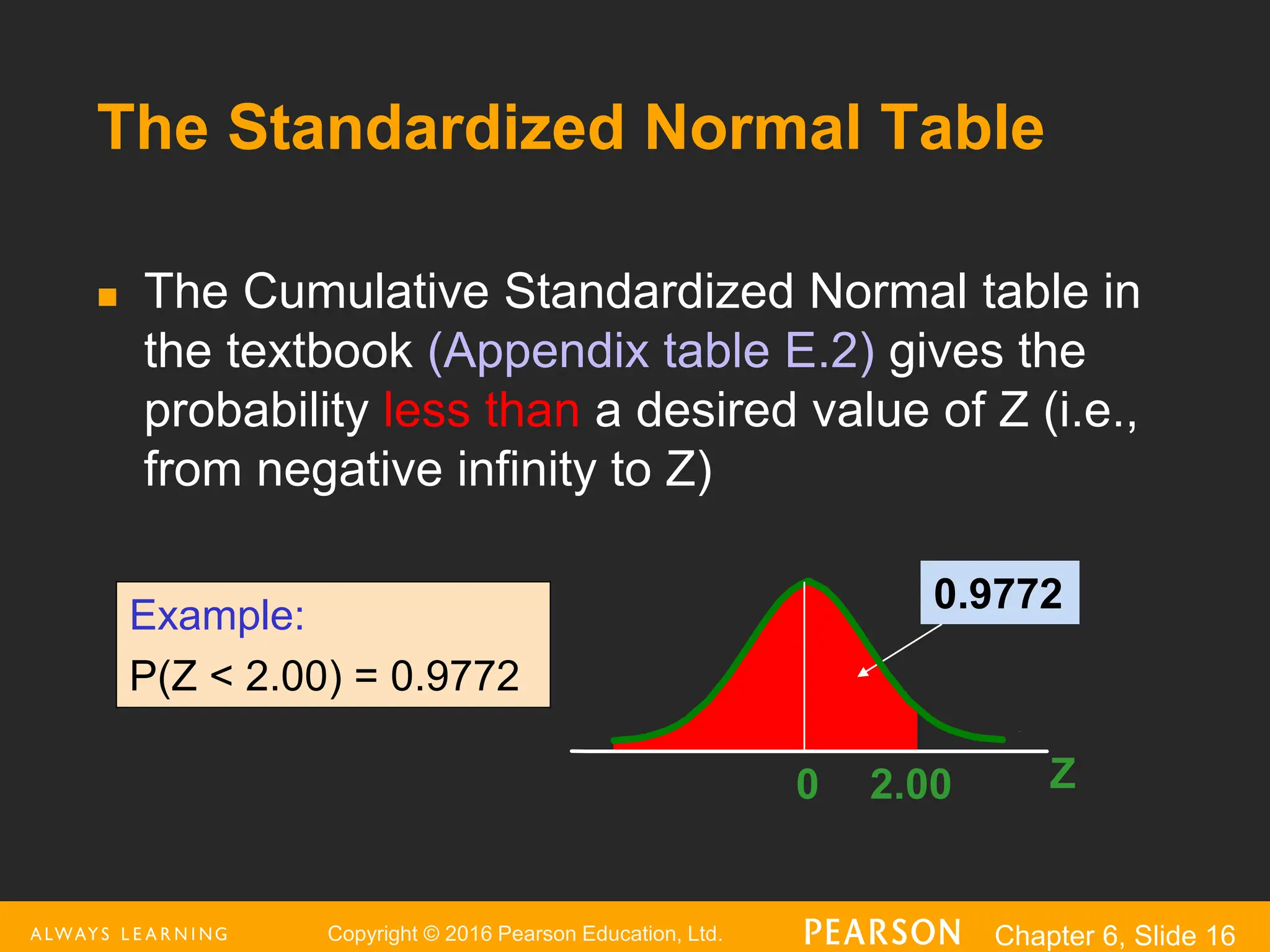
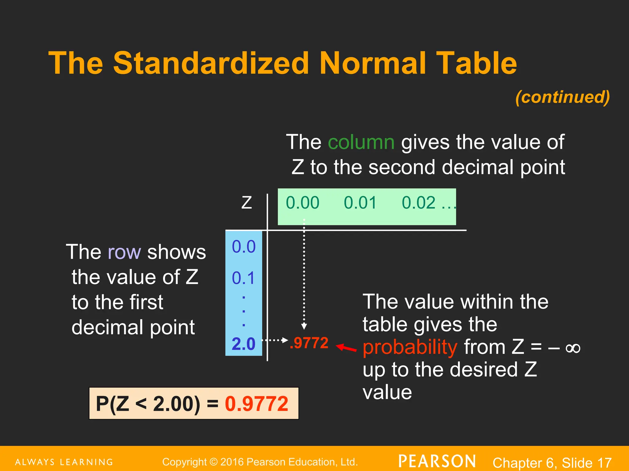
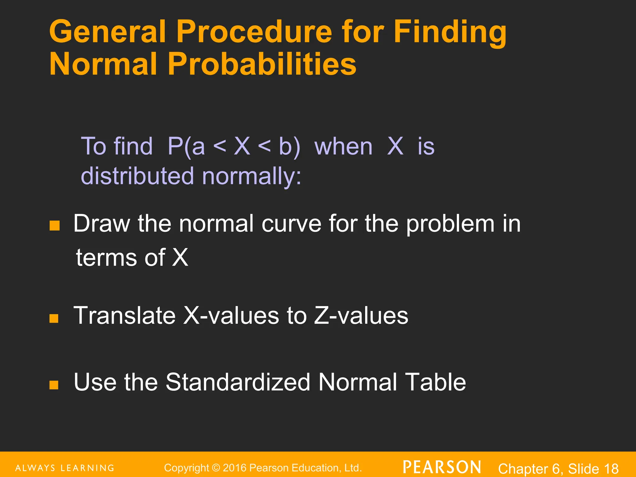
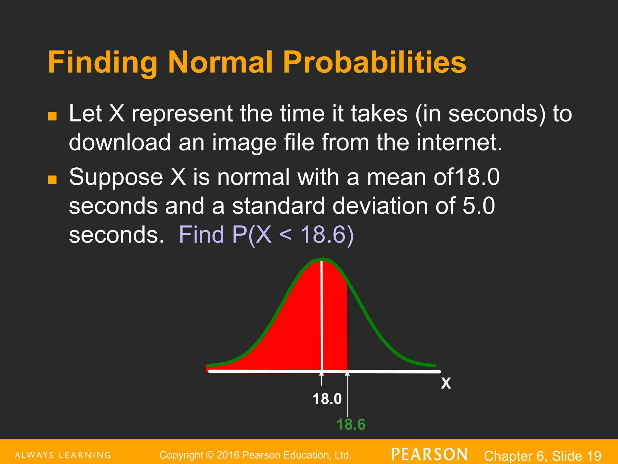
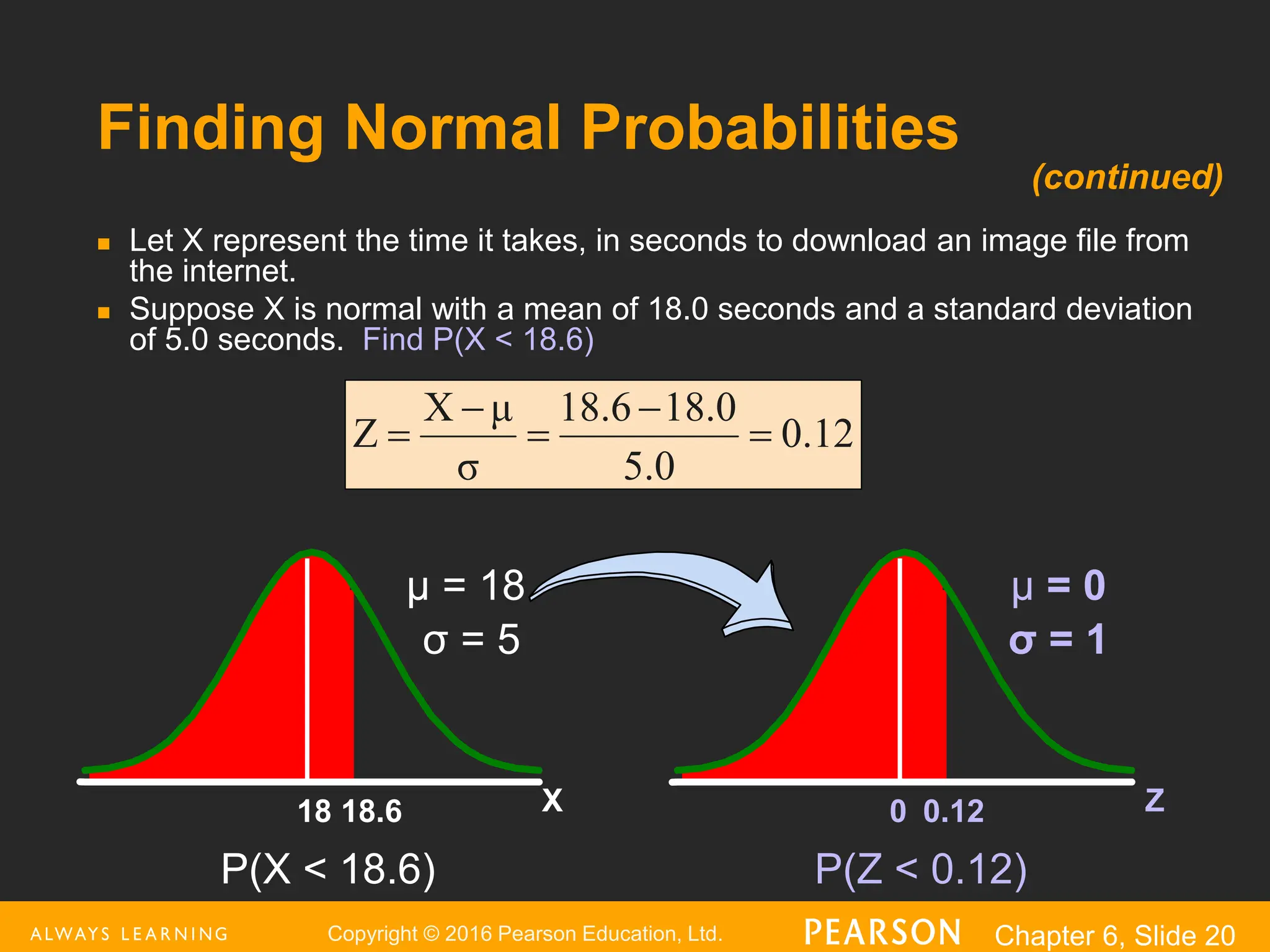
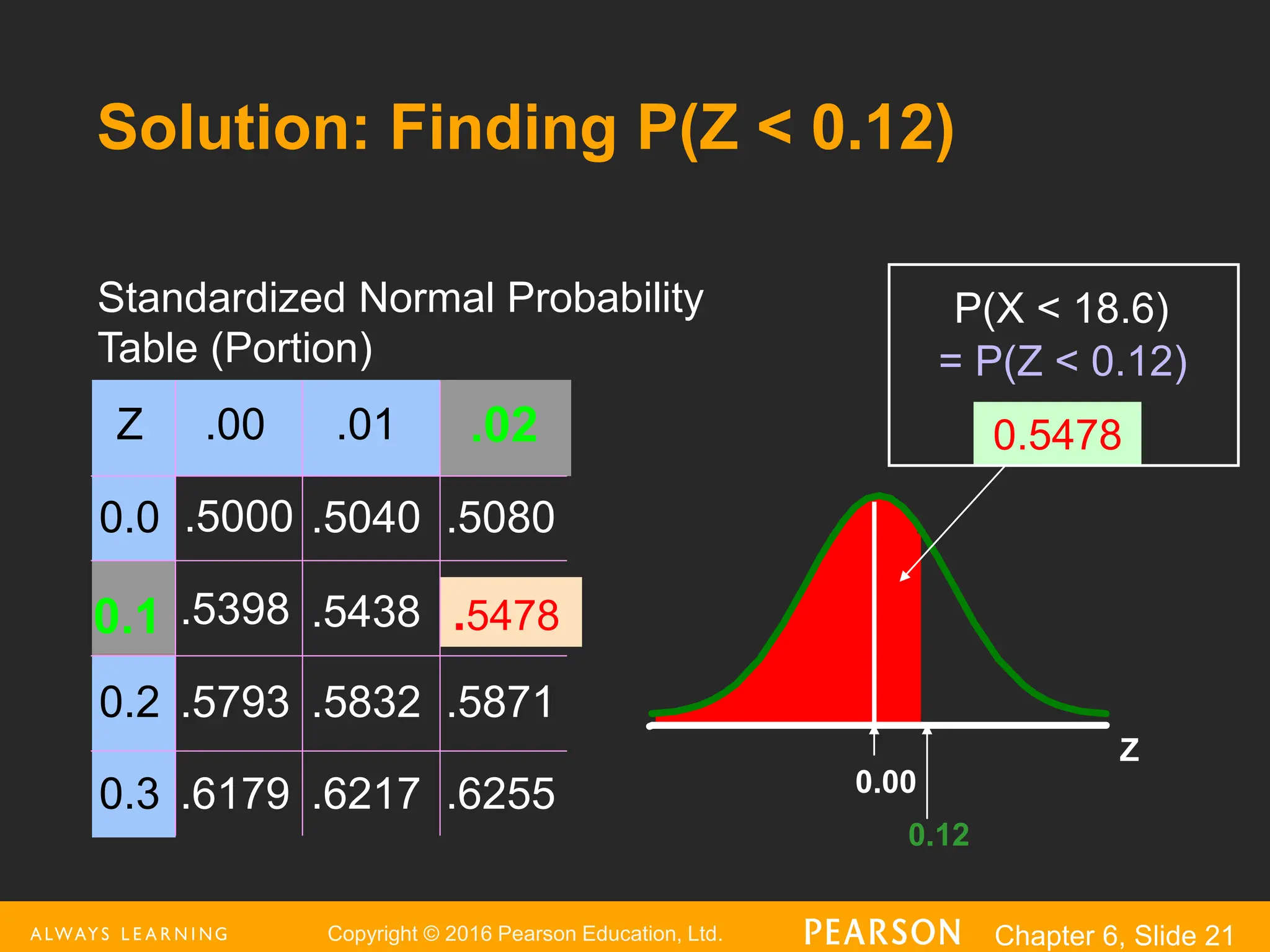
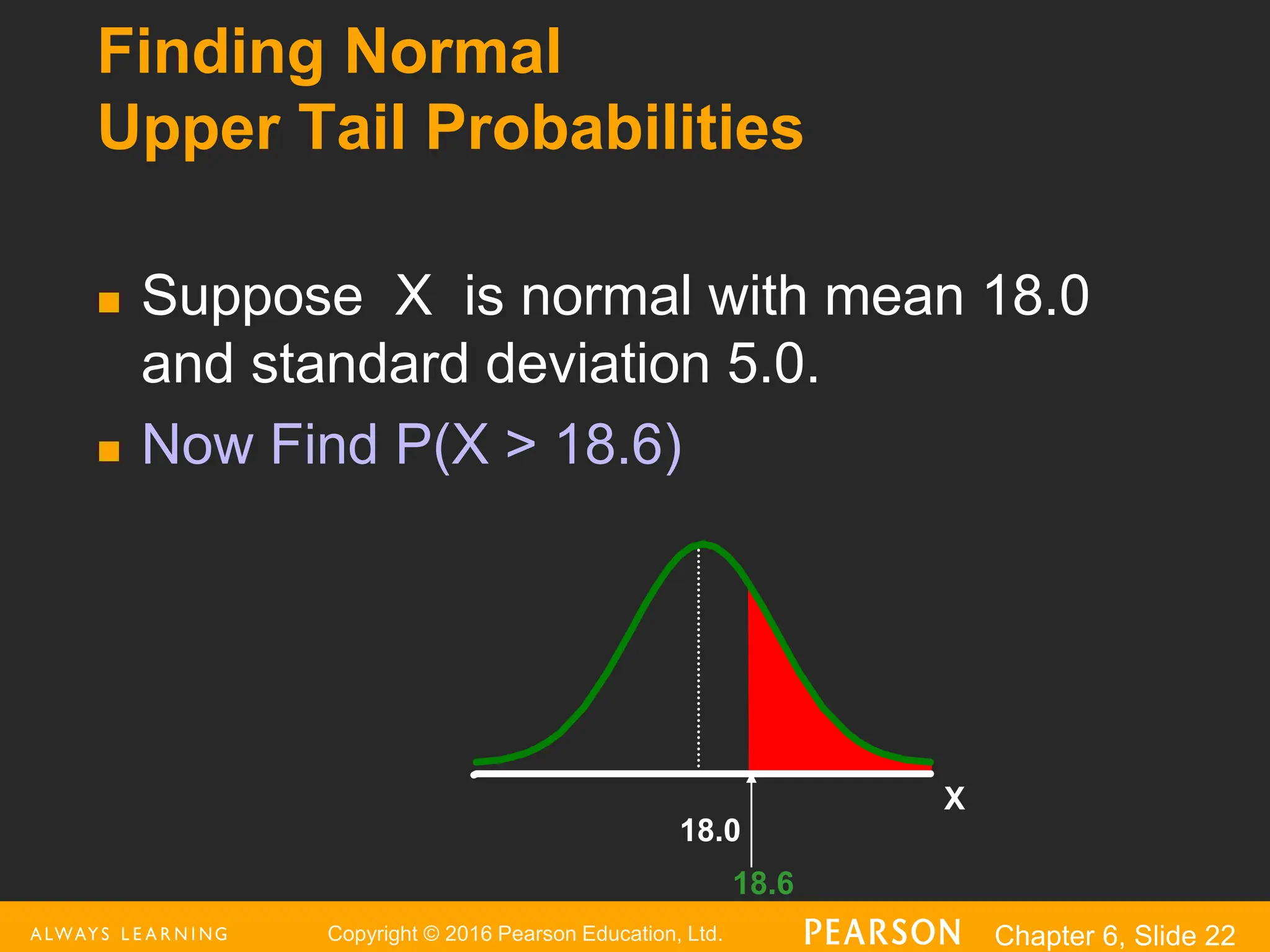
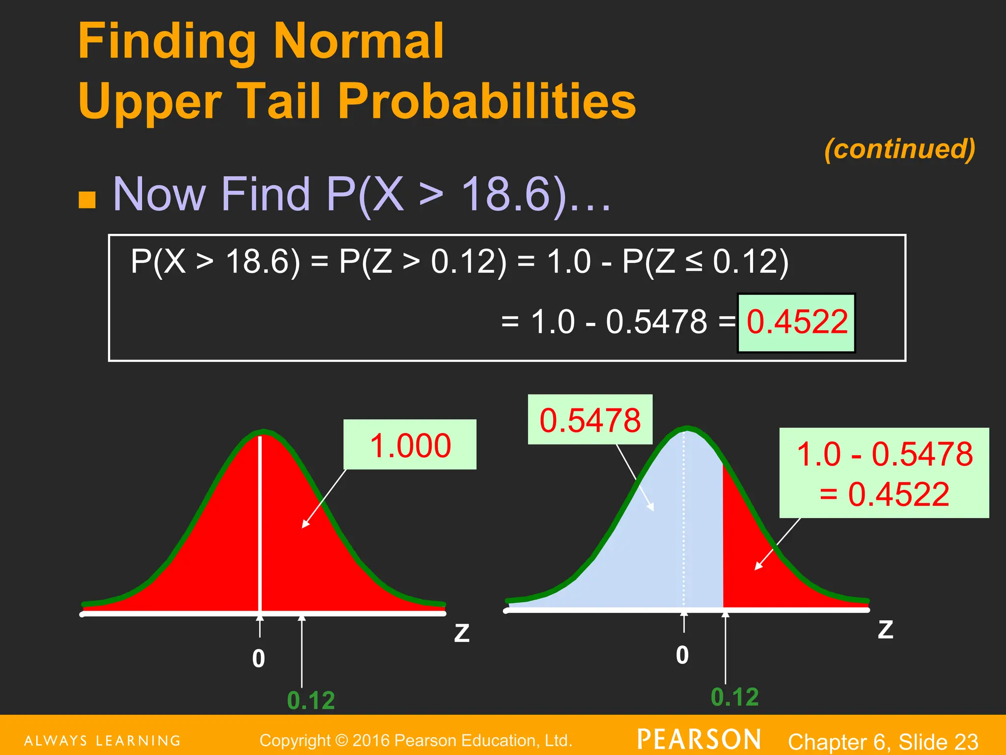
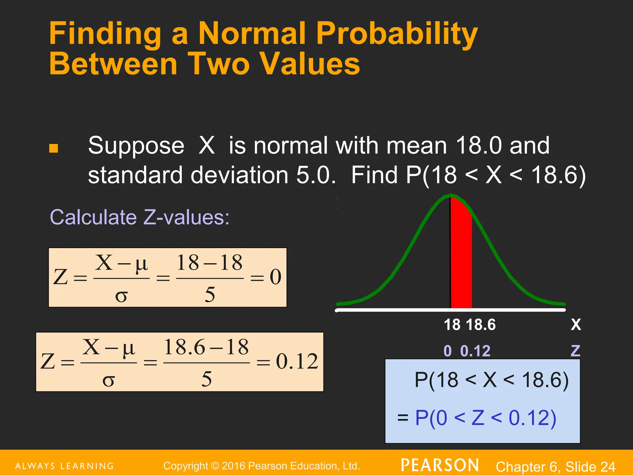
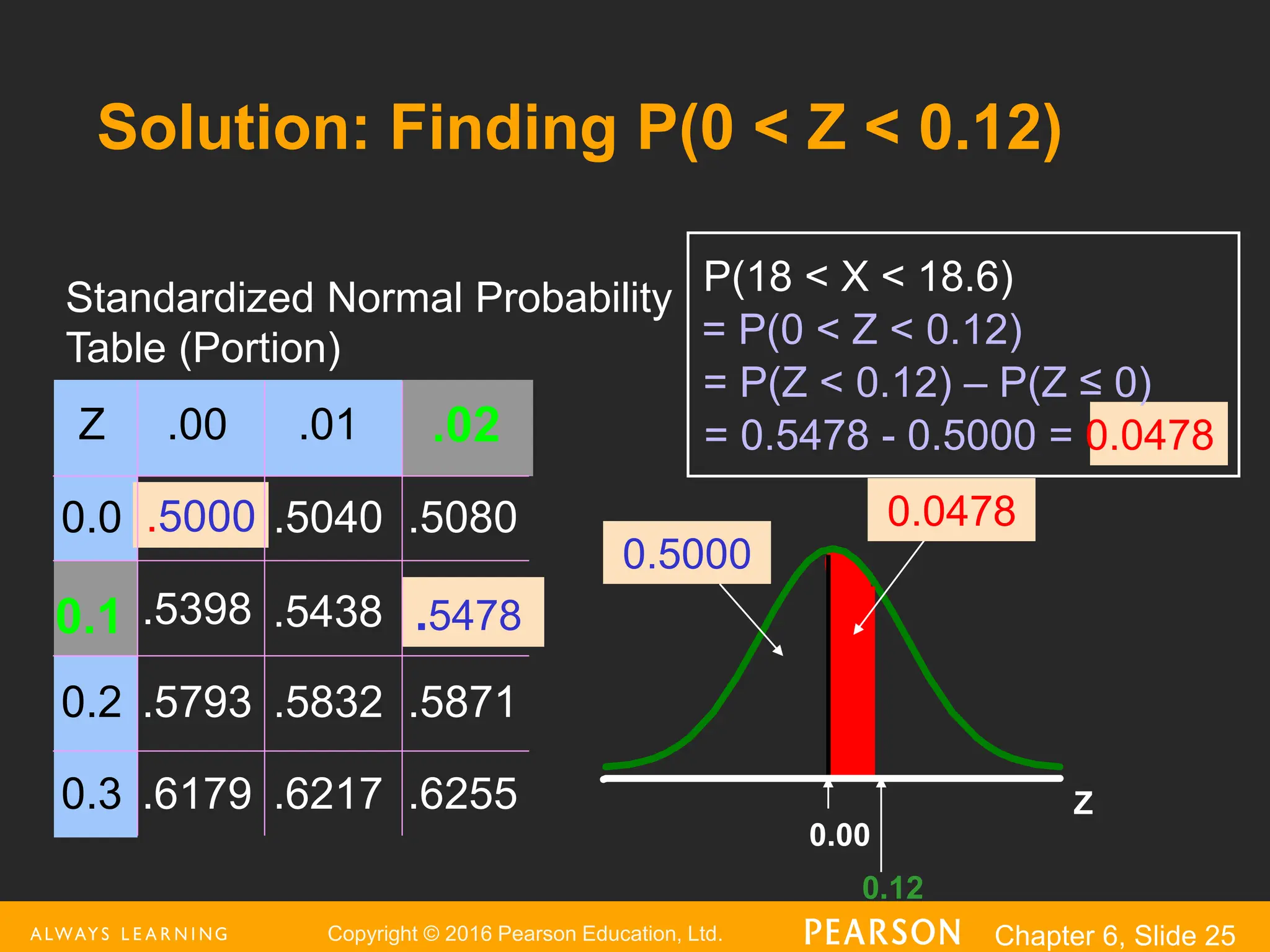
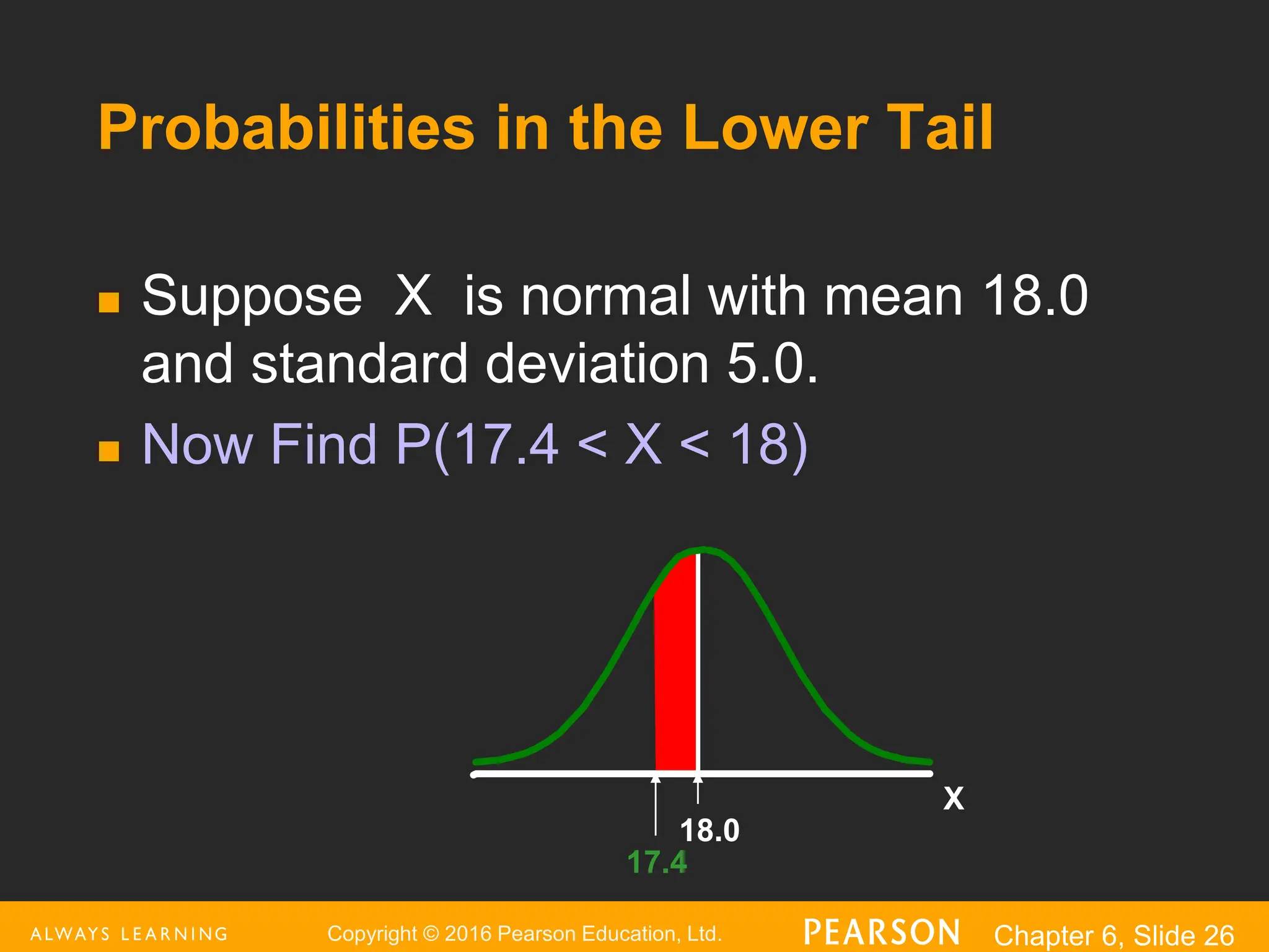
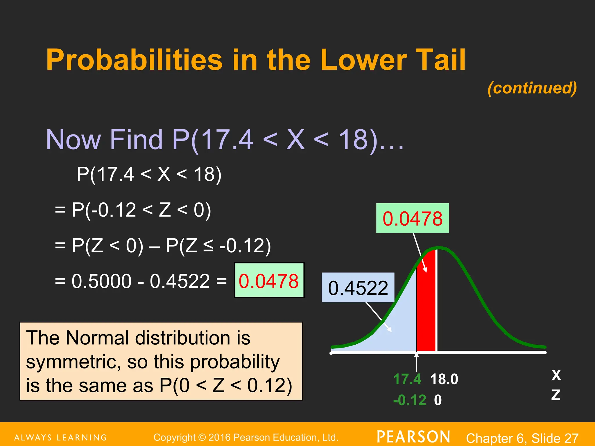
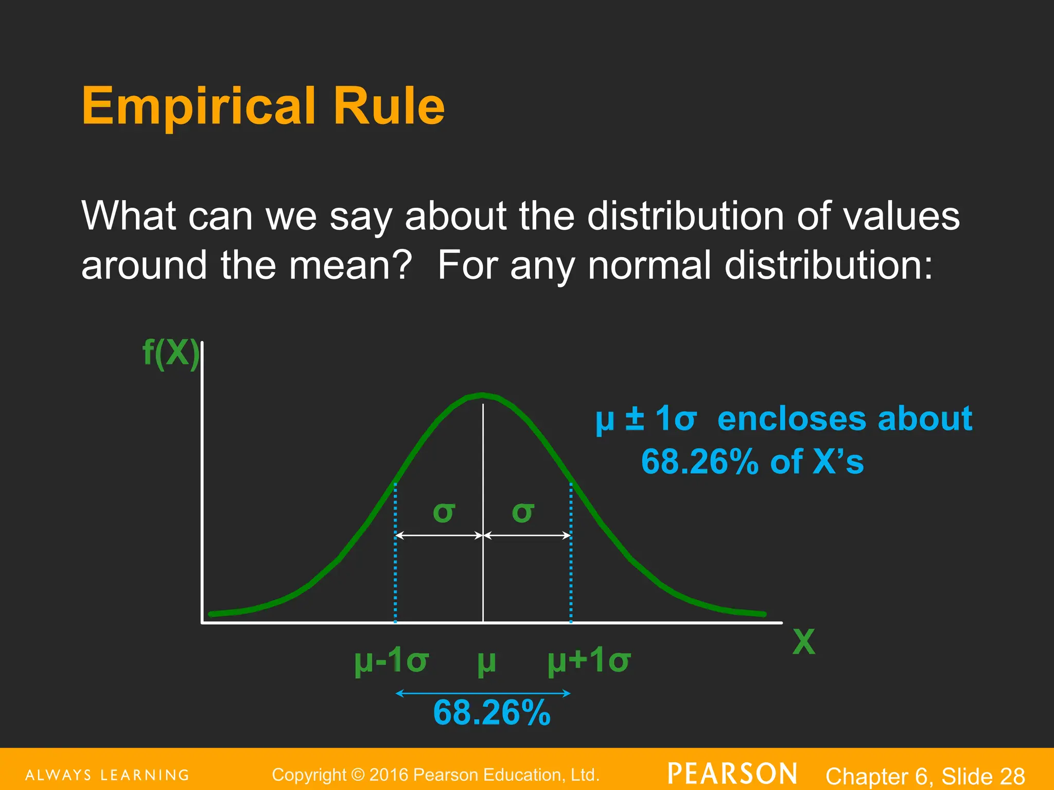
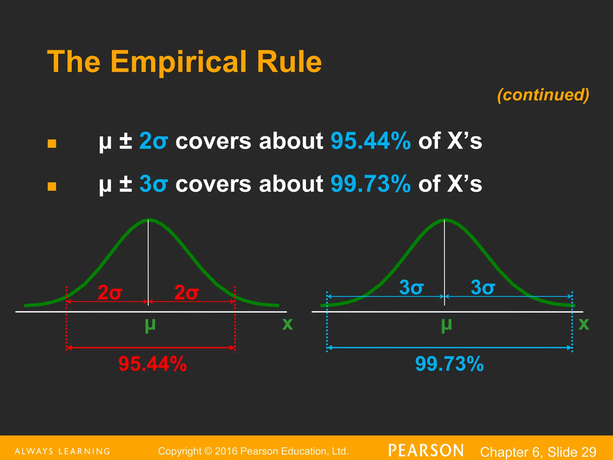
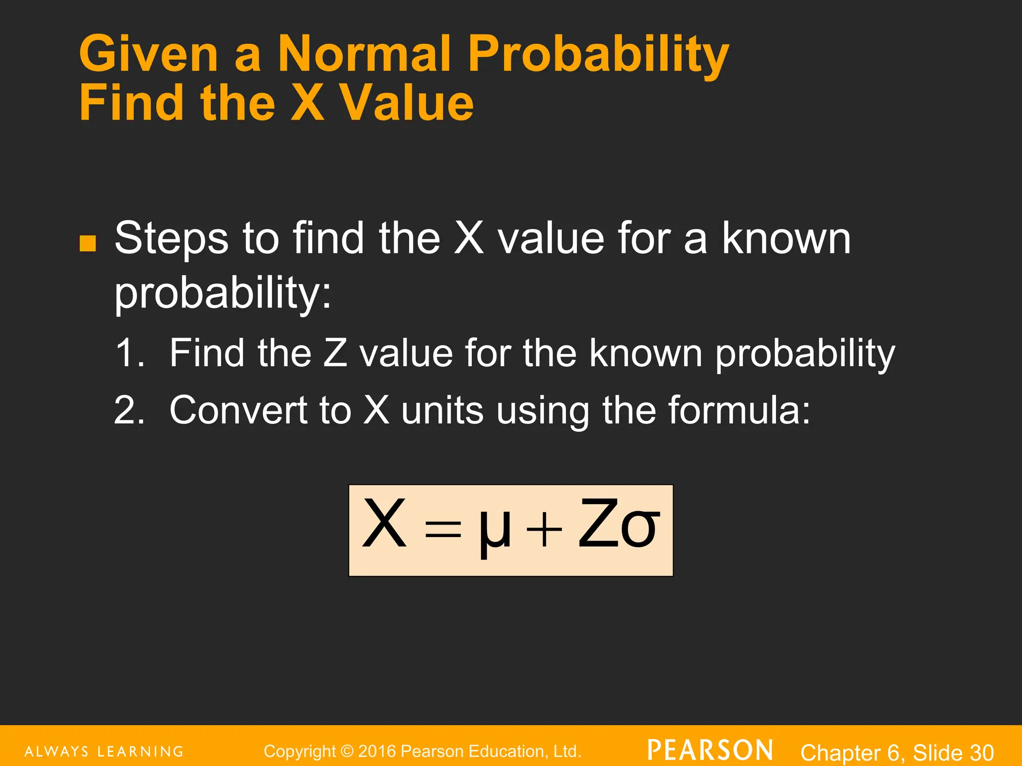
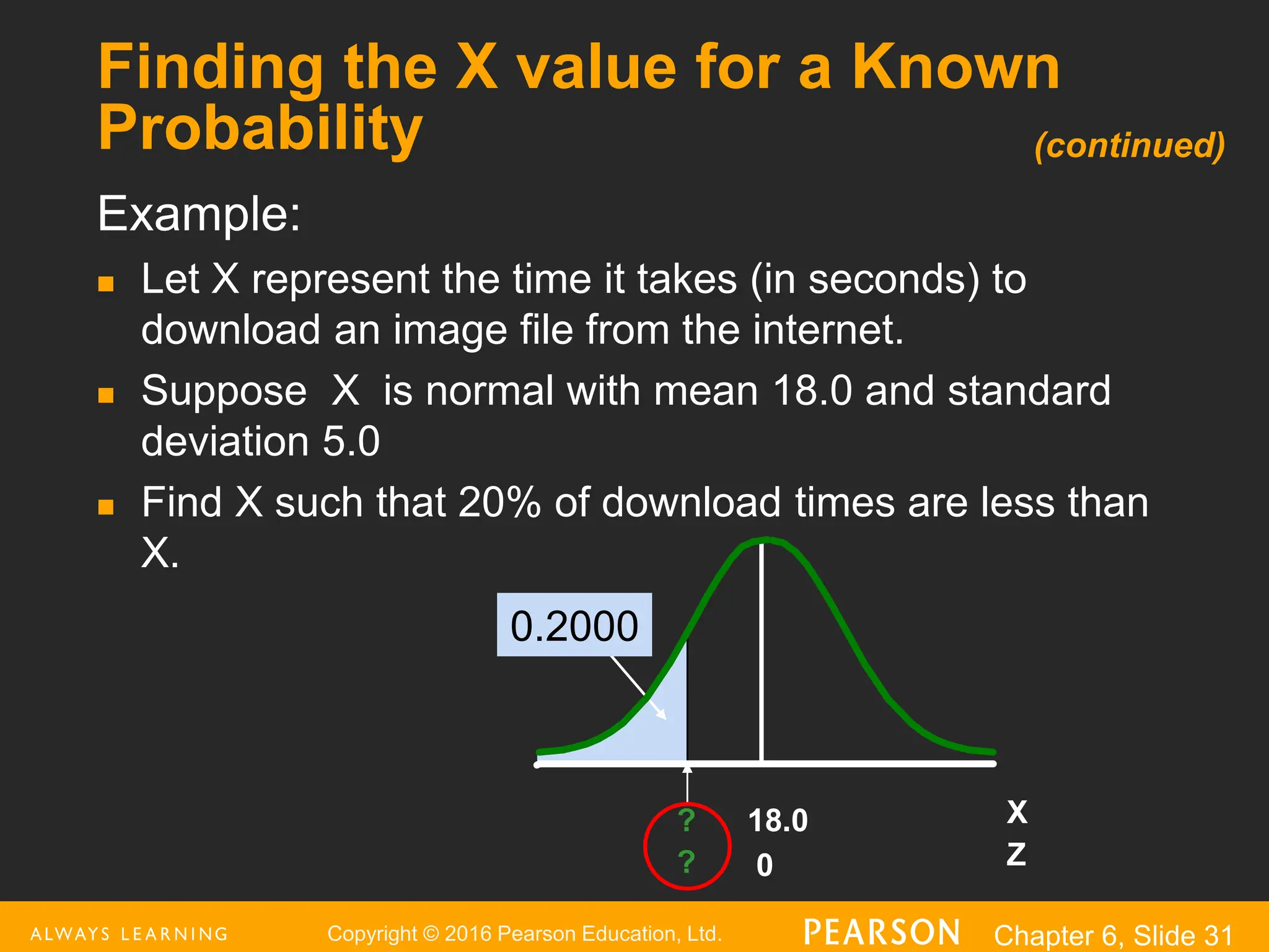
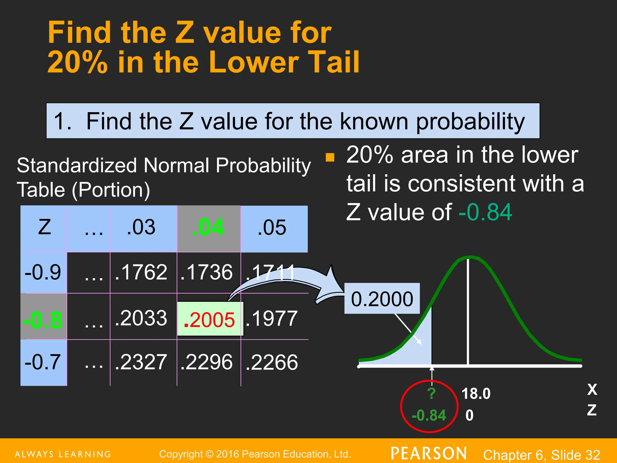
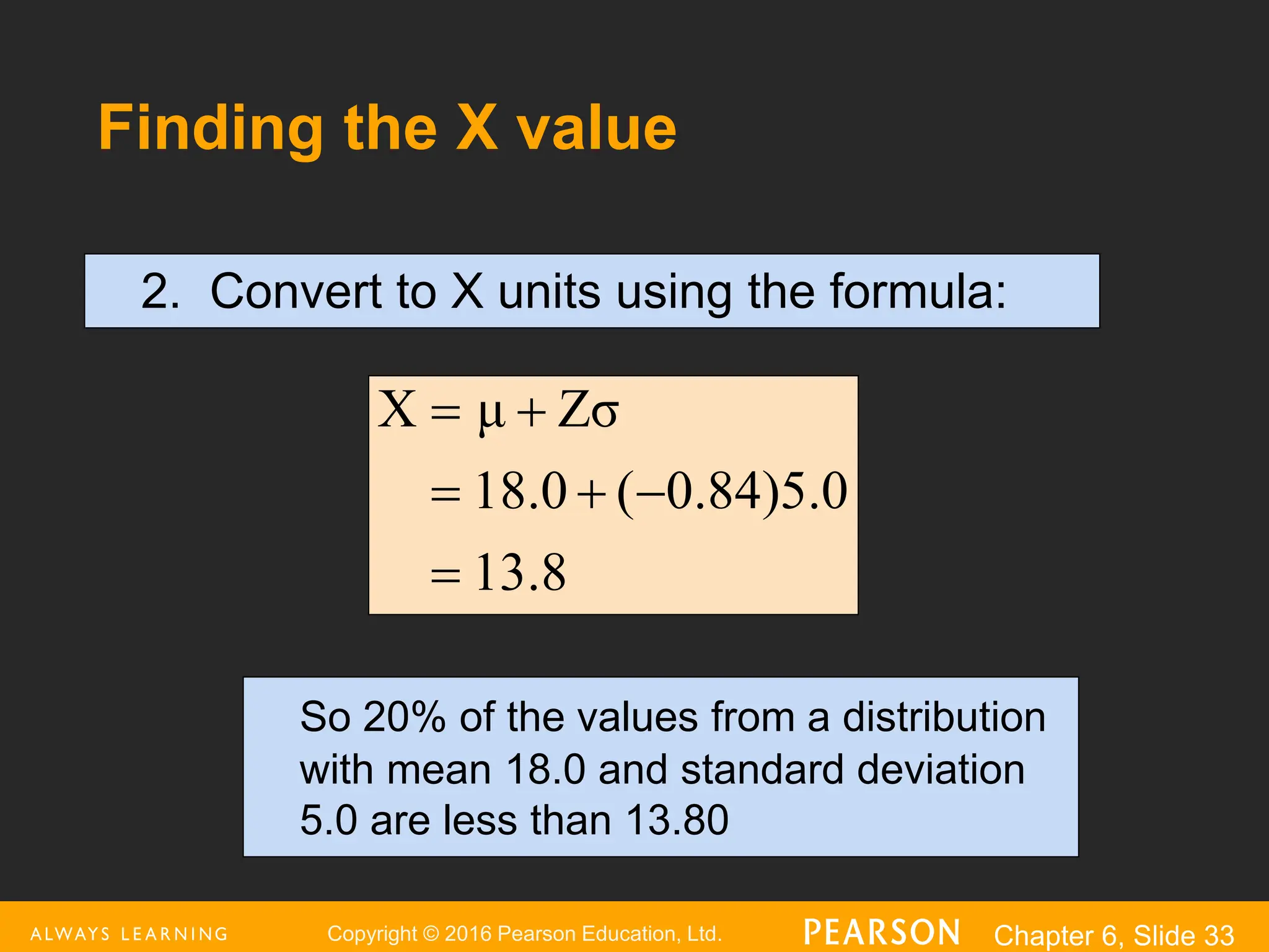
SlideShare a Scribd company logo
Copyright © 2016 Pearson Education, Ltd. Chapter 6, Slide 1
The Normal
Distribution
Chapter 6
Copyright © 2016 Pearson Education, Ltd. Chapter 6, Slide 2
Objectives
In this chapter, you learn:
 To compute probabilities from the normal distribution
 How to use the normal distribution to solve business
problems
 To use the normal probability plot to determine whether
a set of data is approximately normally distributed
Copyright © 2016 Pearson Education, Ltd. Chapter 6, Slide 3
Continuous Probability Distributions
 A continuous variable is a variable that can
assume any value on a continuum (can assume
an uncountable number of values)
 thickness of an item
 time required to complete a task
 temperature of a solution
 height, in inches
 These can potentially take on any value
depending only on the ability to precisely and
accurately measure
Copyright © 2016 Pearson Education, Ltd. Chapter 6, Slide 4
 Bell Shaped
 Symmetrical
 Mean, Median and Mode
are Equal
Location is determined by the
mean, μ
Spread is determined by the
standard deviation, σ
The random variable has an
infinite theoretical range:
+  to  
Mean
= Median
= Mode
X
f(X)
μ
σ
The Normal Distribution
Copyright © 2016 Pearson Education, Ltd. Chapter 6, Slide 5
The Normal Distribution
Density Function
2
μ)
(X
2
1
e
2π
1
f(X)





 

 

 The formula for the normal probability density function is
Where e = the mathematical constant approximated by 2.71828
π = the mathematical constant approximated by 3.14159
μ = the population mean
σ = the population standard deviation
X = any value of the continuous variable
Copyright © 2016 Pearson Education, Ltd. Chapter 6, Slide 6
A
B
C
A and B have the same mean but different standard deviations.
B and C have different means and different standard deviations.
By varying the parameters μ and σ, we
obtain different normal distributions
Copyright © 2016 Pearson Education, Ltd. Chapter 6, Slide 7
The Normal Distribution Shape
X
f(X)
μ
σ
Changing μ shifts the
distribution left or right.
Changing σ increases
or decreases the
spread.
Copyright © 2016 Pearson Education, Ltd. Chapter 6, Slide 8
The Standardized Normal
 Any normal distribution (with any mean and
standard deviation combination) can be
transformed into the standardized normal
distribution (Z)
 To compute normal probabilities need to
transform X units into Z units
 The standardized normal distribution (Z) has a
mean of 0 and a standard deviation of 1
Copyright © 2016 Pearson Education, Ltd. Chapter 6, Slide 9
Translation to the Standardized
Normal Distribution
 Translate from X to the standardized normal
(the “Z” distribution) by subtracting the mean
of X and dividing by its standard deviation:
σ
μ
X
Z


The Z distribution always has mean = 0 and
standard deviation = 1
Copyright © 2016 Pearson Education, Ltd. Chapter 6, Slide 10
The Standardized Normal
Probability Density Function
 The formula for the standardized normal
probability density function is
Where e = the mathematical constant approximated by 2.71828
π = the mathematical constant approximated by 3.14159
Z = any value of the standardized normal distribution
2
(1/2)Z
e
2π
1
f(Z) 

Copyright © 2016 Pearson Education, Ltd. Chapter 6, Slide 11
The Standardized
Normal Distribution
 Also known as the “Z” distribution
 Mean is 0
 Standard Deviation is 1
Z
f(Z)
0
1
Values above the mean have positive Z-values.
Values below the mean have negative Z-values.
Copyright © 2016 Pearson Education, Ltd. Chapter 6, Slide 12
Example
 If X is distributed normally with mean of $100
and standard deviation of $50, the Z value
for X = $200 is
 This says that X = $200 is two standard
deviations (2 increments of $50 units) above
the mean of $100.
2.0
$50
100
$
$200
σ
μ
X
Z 




Copyright © 2016 Pearson Education, Ltd. Chapter 6, Slide 13
Comparing X and Z units
Note that the shape of the distribution is the same,
only the scale has changed. We can express the
problem in the original units (X in dollars) or in
standardized units (Z)
Z
$100
2.0
0
$200 $X(μ = $100, σ = $50)
(μ = 0, σ = 1)
Copyright © 2016 Pearson Education, Ltd. Chapter 6, Slide 14
Probability is measured by the area under
the curve
a b X
f(X) P a X b
( )
≤
≤
P a X b
( )
<
<
=
(Note that the
probability of any
individual value is zero)
Finding Normal Probabilities
Copyright © 2016 Pearson Education, Ltd. Chapter 6, Slide 15
Probability as
Area Under the Curve
The total area under the curve is 1.0, and the curve is
symmetric, so half is above the mean, half is below
f(X)
X
μ
0.5
0.5
1.0
)
X
P( 




0.5
)
X
P(μ 



0.5
μ)
X
P( 



Copyright © 2016 Pearson Education, Ltd. Chapter 6, Slide 16
The Standardized Normal Table
 The Cumulative Standardized Normal table in
the textbook (Appendix table E.2) gives the
probability less than a desired value of Z (i.e.,
from negative infinity to Z)
Z
0 2.00
0.9772
Example:
P(Z < 2.00) = 0.9772
Copyright © 2016 Pearson Education, Ltd. Chapter 6, Slide 17
The Standardized Normal Table
The value within the
table gives the
probability from Z =  
up to the desired Z
value
.9772
2.0
P(Z < 2.00) = 0.9772
The row shows
the value of Z
to the first
decimal point
The column gives the value of
Z to the second decimal point
2.0
.
.
.
(continued)
Z 0.00 0.01 0.02 …
0.0
0.1
Copyright © 2016 Pearson Education, Ltd. Chapter 6, Slide 18
General Procedure for Finding
Normal Probabilities
 Draw the normal curve for the problem in
terms of X
 Translate X-values to Z-values
 Use the Standardized Normal Table
To find P(a < X < b) when X is
distributed normally:
Copyright © 2016 Pearson Education, Ltd. Chapter 6, Slide 19
Finding Normal Probabilities
 Let X represent the time it takes (in seconds) to
download an image file from the internet.
 Suppose X is normal with a mean of18.0
seconds and a standard deviation of 5.0
seconds. Find P(X < 18.6)
18.6
X
18.0
Copyright © 2016 Pearson Education, Ltd. Chapter 6, Slide 20
Finding Normal Probabilities
 Let X represent the time it takes, in seconds to download an image file from
the internet.
 Suppose X is normal with a mean of 18.0 seconds and a standard deviation
of 5.0 seconds. Find P(X < 18.6)
Z
0.12
0
X
18.6
18
μ = 18
σ = 5
μ = 0
σ = 1
(continued)
0.12
5.0
8.0
1
18.6
σ
μ
X
Z 




P(X < 18.6) P(Z < 0.12)
Copyright © 2016 Pearson Education, Ltd. Chapter 6, Slide 21
Z
0.12
0.5478
Standardized Normal Probability
Table (Portion)
0.00
= P(Z < 0.12)
P(X < 18.6)
Z .00 .01
0.0 .5000 .5040 .5080
.5398 .5438
0.2 .5793 .5832 .5871
0.3 .6179 .6217 .6255
.02
0.1 .5478
Solution: Finding P(Z < 0.12)
Copyright © 2016 Pearson Education, Ltd. Chapter 6, Slide 22
Finding Normal
Upper Tail Probabilities
 Suppose X is normal with mean 18.0
and standard deviation 5.0.
 Now Find P(X > 18.6)
X
18.6
18.0
Copyright © 2016 Pearson Education, Ltd. Chapter 6, Slide 23
Finding Normal
Upper Tail Probabilities
 Now Find P(X > 18.6)…
(continued)
Z
0.12
0
Z
0.12
0.5478
0
1.000 1.0 - 0.5478
= 0.4522
P(X > 18.6) = P(Z > 0.12) = 1.0 - P(Z ≤ 0.12)
= 1.0 - 0.5478 = 0.4522
Copyright © 2016 Pearson Education, Ltd. Chapter 6, Slide 24
Finding a Normal Probability
Between Two Values
 Suppose X is normal with mean 18.0 and
standard deviation 5.0. Find P(18 < X < 18.6)
P(18 < X < 18.6)
= P(0 < Z < 0.12)
Z
0.12
0
X
18.6
18
0
5
8
1
18
σ
μ
X
Z 




0.12
5
8
1
18.6
σ
μ
X
Z 




Calculate Z-values:
Copyright © 2016 Pearson Education, Ltd. Chapter 6, Slide 25
Z
0.12
0.0478
0.00
= P(0 < Z < 0.12)
P(18 < X < 18.6)
= P(Z < 0.12) – P(Z ≤ 0)
= 0.5478 - 0.5000 = 0.0478
0.5000
Z .00 .01
0.0 .5000 .5040 .5080
.5398 .5438
0.2 .5793 .5832 .5871
0.3 .6179 .6217 .6255
.02
0.1 .5478
Standardized Normal Probability
Table (Portion)
Solution: Finding P(0 < Z < 0.12)
Copyright © 2016 Pearson Education, Ltd. Chapter 6, Slide 26
Probabilities in the Lower Tail
 Suppose X is normal with mean 18.0
and standard deviation 5.0.
 Now Find P(17.4 < X < 18)
X
17.4
18.0
Copyright © 2016 Pearson Education, Ltd. Chapter 6, Slide 27
Probabilities in the Lower Tail
Now Find P(17.4 < X < 18)…
X
17.4 18.0
P(17.4 < X < 18)
= P(-0.12 < Z < 0)
= P(Z < 0) – P(Z ≤ -0.12)
= 0.5000 - 0.4522 = 0.0478
(continued)
0.0478
0.4522
Z
-0.12 0
The Normal distribution is
symmetric, so this probability
is the same as P(0 < Z < 0.12)
Copyright © 2016 Pearson Education, Ltd. Chapter 6, Slide 28
Empirical Rule
μ ± 1σ encloses about
68.26% of X’s
f(X)
X
μ μ+1σ
μ-1σ
What can we say about the distribution of values
around the mean? For any normal distribution:
σ
σ
68.26%
Copyright © 2016 Pearson Education, Ltd. Chapter 6, Slide 29
The Empirical Rule
 μ ± 2σ covers about 95.44% of X’s
 μ ± 3σ covers about 99.73% of X’s
x
μ
2σ 2σ
x
μ
3σ 3σ
95.44% 99.73%
(continued)
Copyright © 2016 Pearson Education, Ltd. Chapter 6, Slide 30
Given a Normal Probability
Find the X Value
 Steps to find the X value for a known
probability:
1. Find the Z value for the known probability
2. Convert to X units using the formula:
Zσ
μ
X 

Copyright © 2016 Pearson Education, Ltd. Chapter 6, Slide 31
Finding the X value for a Known
Probability
Example:
 Let X represent the time it takes (in seconds) to
download an image file from the internet.
 Suppose X is normal with mean 18.0 and standard
deviation 5.0
 Find X such that 20% of download times are less than
X.
X
? 18.0
0.2000
Z
? 0
(continued)
Copyright © 2016 Pearson Education, Ltd. Chapter 6, Slide 32
Find the Z value for
20% in the Lower Tail
 20% area in the lower
tail is consistent with a
Z value of -0.84
Z .03
-0.9 .1762 .1736
.2033
-0.7 .2327 .2296
.04
-0.8 .2005
Standardized Normal Probability
Table (Portion)
.05
.1711
.1977
.2266
…
…
…
…
X
? 18.0
0.2000
Z
-0.84 0
1. Find the Z value for the known probability
Copyright © 2016 Pearson Education, Ltd. Chapter 6, Slide 33
Finding the X value
2. Convert to X units using the formula:
8
.
13
0
.
5
)
84
.
0
(
0
.
18
Zσ
μ
X






So 20% of the values from a distribution
with mean 18.0 and standard deviation
5.0 are less than 13.80
Copyright © 2016 Pearson Education, Ltd. Chapter 6, Slide 34
Chapter Summary
In this chapter we discussed:
 Computing probabilities from the normal distribution
 Using the normal distribution to solve business
problems
 Using the normal probability plot to determine whether a
set of data is approximately normally distributed

More Related Content

Similar to normal distribution_normal distribution_

Chapter16 continuousrandomvariables-151007043951-lva1-app6892
Chapter16 continuousrandomvariables-151007043951-lva1-app6892Chapter16 continuousrandomvariables-151007043951-lva1-app6892
Chapter16 continuousrandomvariables-151007043951-lva1-app6892
Cleophas Rwemera
 
Introductory maths analysis chapter 16 official
Introductory maths analysis   chapter 16 officialIntroductory maths analysis   chapter 16 official
Introductory maths analysis chapter 16 official
Evert Sandye Taasiringan
 
Chapter 16 - Continuous Random Variables
Chapter 16 - Continuous Random VariablesChapter 16 - Continuous Random Variables
Chapter 16 - Continuous Random Variables
Muhammad Bilal Khairuddin
 
Applied Business Statistics ,ken black , ch 6
Applied Business Statistics ,ken black , ch 6Applied Business Statistics ,ken black , ch 6
Applied Business Statistics ,ken black , ch 6
AbdelmonsifFadl
 
raghu veera stats.ppt
raghu veera stats.pptraghu veera stats.ppt
raghu veera stats.ppt
DevarajuBn
 
Statistik 1 6 distribusi probabilitas normal
Statistik 1 6 distribusi probabilitas normalStatistik 1 6 distribusi probabilitas normal
Statistik 1 6 distribusi probabilitas normalSelvin Hadi
 
L6.slides.pdf
L6.slides.pdfL6.slides.pdf
L6.slides.pdf
ssuser953ee81
 
L6.slides.pdf
L6.slides.pdfL6.slides.pdf
L6.slides.pdf
ssuser953ee81
 
Discrete and continuous probability distributions ppt @ bec doms
Discrete and continuous probability distributions ppt @ bec domsDiscrete and continuous probability distributions ppt @ bec doms
Discrete and continuous probability distributions ppt @ bec doms
Babasab Patil
 
Chap06 normal distributions & continous
Chap06 normal distributions & continousChap06 normal distributions & continous
Chap06 normal distributions & continous
Uni Azza Aunillah
 
Applied Business Statistics ,ken black , ch 5
Applied Business Statistics ,ken black , ch 5Applied Business Statistics ,ken black , ch 5
Applied Business Statistics ,ken black , ch 5
AbdelmonsifFadl
 
Lec. 10: Making Assumptions of Missing data
Lec. 10: Making Assumptions of Missing dataLec. 10: Making Assumptions of Missing data
Lec. 10: Making Assumptions of Missing data
MohamadKharseh1
 
Chapter 6 2022.pdf
Chapter 6 2022.pdfChapter 6 2022.pdf
Chapter 6 2022.pdf
Mohamed Ali
 
Options Portfolio Selection
Options Portfolio SelectionOptions Portfolio Selection
Options Portfolio Selection
guasoni
 
Normal Distribution.pdf
Normal Distribution.pdfNormal Distribution.pdf
Normal Distribution.pdf
RAHULSUTHAR46
 
Real Applications of Normal Distributions
Real Applications of Normal Distributions  Real Applications of Normal Distributions
Real Applications of Normal Distributions
Long Beach City College
 
Binomial probability distributions
Binomial probability distributions  Binomial probability distributions
Binomial probability distributions
Long Beach City College
 
BBS10_ppt_ch07_Sampling_Distribution.ppt
BBS10_ppt_ch07_Sampling_Distribution.pptBBS10_ppt_ch07_Sampling_Distribution.ppt
BBS10_ppt_ch07_Sampling_Distribution.ppt
Hermita3
 
Quantitative Methods for Lawyers - Class #10 - Binomial Distributions, Normal...
Quantitative Methods for Lawyers - Class #10 - Binomial Distributions, Normal...Quantitative Methods for Lawyers - Class #10 - Binomial Distributions, Normal...
Quantitative Methods for Lawyers - Class #10 - Binomial Distributions, Normal...
Daniel Katz
 

Similar to normal distribution_normal distribution_ (20)

Chapter16 continuousrandomvariables-151007043951-lva1-app6892
Chapter16 continuousrandomvariables-151007043951-lva1-app6892Chapter16 continuousrandomvariables-151007043951-lva1-app6892
Chapter16 continuousrandomvariables-151007043951-lva1-app6892
 
Introductory maths analysis chapter 16 official
Introductory maths analysis   chapter 16 officialIntroductory maths analysis   chapter 16 official
Introductory maths analysis chapter 16 official
 
Chapter 16 - Continuous Random Variables
Chapter 16 - Continuous Random VariablesChapter 16 - Continuous Random Variables
Chapter 16 - Continuous Random Variables
 
Applied Business Statistics ,ken black , ch 6
Applied Business Statistics ,ken black , ch 6Applied Business Statistics ,ken black , ch 6
Applied Business Statistics ,ken black , ch 6
 
raghu veera stats.ppt
raghu veera stats.pptraghu veera stats.ppt
raghu veera stats.ppt
 
Statistik 1 6 distribusi probabilitas normal
Statistik 1 6 distribusi probabilitas normalStatistik 1 6 distribusi probabilitas normal
Statistik 1 6 distribusi probabilitas normal
 
L6.slides.pdf
L6.slides.pdfL6.slides.pdf
L6.slides.pdf
 
L6.slides.pdf
L6.slides.pdfL6.slides.pdf
L6.slides.pdf
 
Discrete and continuous probability distributions ppt @ bec doms
Discrete and continuous probability distributions ppt @ bec domsDiscrete and continuous probability distributions ppt @ bec doms
Discrete and continuous probability distributions ppt @ bec doms
 
Chap06 normal distributions & continous
Chap06 normal distributions & continousChap06 normal distributions & continous
Chap06 normal distributions & continous
 
Applied Business Statistics ,ken black , ch 5
Applied Business Statistics ,ken black , ch 5Applied Business Statistics ,ken black , ch 5
Applied Business Statistics ,ken black , ch 5
 
Lec. 10: Making Assumptions of Missing data
Lec. 10: Making Assumptions of Missing dataLec. 10: Making Assumptions of Missing data
Lec. 10: Making Assumptions of Missing data
 
Chapter 6 2022.pdf
Chapter 6 2022.pdfChapter 6 2022.pdf
Chapter 6 2022.pdf
 
Options Portfolio Selection
Options Portfolio SelectionOptions Portfolio Selection
Options Portfolio Selection
 
Normal Distribution.pdf
Normal Distribution.pdfNormal Distribution.pdf
Normal Distribution.pdf
 
Normal Distribution
Normal DistributionNormal Distribution
Normal Distribution
 
Real Applications of Normal Distributions
Real Applications of Normal Distributions  Real Applications of Normal Distributions
Real Applications of Normal Distributions
 
Binomial probability distributions
Binomial probability distributions  Binomial probability distributions
Binomial probability distributions
 
BBS10_ppt_ch07_Sampling_Distribution.ppt
BBS10_ppt_ch07_Sampling_Distribution.pptBBS10_ppt_ch07_Sampling_Distribution.ppt
BBS10_ppt_ch07_Sampling_Distribution.ppt
 
Quantitative Methods for Lawyers - Class #10 - Binomial Distributions, Normal...
Quantitative Methods for Lawyers - Class #10 - Binomial Distributions, Normal...Quantitative Methods for Lawyers - Class #10 - Binomial Distributions, Normal...
Quantitative Methods for Lawyers - Class #10 - Binomial Distributions, Normal...
 

Recently uploaded

road safety engineering r s e unit 3.pdf
road safety engineering  r s e unit 3.pdfroad safety engineering  r s e unit 3.pdf
road safety engineering r s e unit 3.pdf
VENKATESHvenky89705
 
LIGA(E)11111111111111111111111111111111111111111.ppt
LIGA(E)11111111111111111111111111111111111111111.pptLIGA(E)11111111111111111111111111111111111111111.ppt
LIGA(E)11111111111111111111111111111111111111111.ppt
ssuser9bd3ba
 
addressing modes in computer architecture
addressing modes  in computer architectureaddressing modes  in computer architecture
addressing modes in computer architecture
ShahidSultan24
 
H.Seo, ICLR 2024, MLILAB, KAIST AI.pdf
H.Seo,  ICLR 2024, MLILAB,  KAIST AI.pdfH.Seo,  ICLR 2024, MLILAB,  KAIST AI.pdf
H.Seo, ICLR 2024, MLILAB, KAIST AI.pdf
MLILAB
 
ASME IX(9) 2007 Full Version .pdf
ASME IX(9)  2007 Full Version       .pdfASME IX(9)  2007 Full Version       .pdf
ASME IX(9) 2007 Full Version .pdf
AhmedHussein950959
 
Gen AI Study Jams _ For the GDSC Leads in India.pdf
Gen AI Study Jams _ For the GDSC Leads in India.pdfGen AI Study Jams _ For the GDSC Leads in India.pdf
Gen AI Study Jams _ For the GDSC Leads in India.pdf
gdsczhcet
 
TECHNICAL TRAINING MANUAL GENERAL FAMILIARIZATION COURSE
TECHNICAL TRAINING MANUAL   GENERAL FAMILIARIZATION COURSETECHNICAL TRAINING MANUAL   GENERAL FAMILIARIZATION COURSE
TECHNICAL TRAINING MANUAL GENERAL FAMILIARIZATION COURSE
DuvanRamosGarzon1
 
MCQ Soil mechanics questions (Soil shear strength).pdf
MCQ Soil mechanics questions (Soil shear strength).pdfMCQ Soil mechanics questions (Soil shear strength).pdf
MCQ Soil mechanics questions (Soil shear strength).pdf
Osamah Alsalih
 
Student information management system project report ii.pdf
Student information management system project report ii.pdfStudent information management system project report ii.pdf
Student information management system project report ii.pdf
Kamal Acharya
 
Sachpazis:Terzaghi Bearing Capacity Estimation in simple terms with Calculati...
Sachpazis:Terzaghi Bearing Capacity Estimation in simple terms with Calculati...Sachpazis:Terzaghi Bearing Capacity Estimation in simple terms with Calculati...
Sachpazis:Terzaghi Bearing Capacity Estimation in simple terms with Calculati...
Dr.Costas Sachpazis
 
Architectural Portfolio Sean Lockwood
Architectural Portfolio Sean LockwoodArchitectural Portfolio Sean Lockwood
Architectural Portfolio Sean Lockwood
seandesed
 
HYDROPOWER - Hydroelectric power generation
HYDROPOWER - Hydroelectric power generationHYDROPOWER - Hydroelectric power generation
HYDROPOWER - Hydroelectric power generation
Robbie Edward Sayers
 
Halogenation process of chemical process industries
Halogenation process of chemical process industriesHalogenation process of chemical process industries
Halogenation process of chemical process industries
MuhammadTufail242431
 
Top 10 Oil and Gas Projects in Saudi Arabia 2024.pdf
Top 10 Oil and Gas Projects in Saudi Arabia 2024.pdfTop 10 Oil and Gas Projects in Saudi Arabia 2024.pdf
Top 10 Oil and Gas Projects in Saudi Arabia 2024.pdf
Teleport Manpower Consultant
 
NO1 Uk best vashikaran specialist in delhi vashikaran baba near me online vas...
NO1 Uk best vashikaran specialist in delhi vashikaran baba near me online vas...NO1 Uk best vashikaran specialist in delhi vashikaran baba near me online vas...
NO1 Uk best vashikaran specialist in delhi vashikaran baba near me online vas...
Amil Baba Dawood bangali
 
Design and Analysis of Algorithms-DP,Backtracking,Graphs,B&B
Design and Analysis of Algorithms-DP,Backtracking,Graphs,B&BDesign and Analysis of Algorithms-DP,Backtracking,Graphs,B&B
Design and Analysis of Algorithms-DP,Backtracking,Graphs,B&B
Sreedhar Chowdam
 
CME397 Surface Engineering- Professional Elective
CME397 Surface Engineering- Professional ElectiveCME397 Surface Engineering- Professional Elective
CME397 Surface Engineering- Professional Elective
karthi keyan
 
一比一原版(SFU毕业证)西蒙菲莎大学毕业证成绩单如何办理
一比一原版(SFU毕业证)西蒙菲莎大学毕业证成绩单如何办理一比一原版(SFU毕业证)西蒙菲莎大学毕业证成绩单如何办理
一比一原版(SFU毕业证)西蒙菲莎大学毕业证成绩单如何办理
bakpo1
 
power quality voltage fluctuation UNIT - I.pptx
power quality voltage fluctuation UNIT - I.pptxpower quality voltage fluctuation UNIT - I.pptx
power quality voltage fluctuation UNIT - I.pptx
ViniHema
 
Nuclear Power Economics and Structuring 2024
Nuclear Power Economics and Structuring 2024Nuclear Power Economics and Structuring 2024
Nuclear Power Economics and Structuring 2024
Massimo Talia
 

Recently uploaded (20)

road safety engineering r s e unit 3.pdf
road safety engineering  r s e unit 3.pdfroad safety engineering  r s e unit 3.pdf
road safety engineering r s e unit 3.pdf
 
LIGA(E)11111111111111111111111111111111111111111.ppt
LIGA(E)11111111111111111111111111111111111111111.pptLIGA(E)11111111111111111111111111111111111111111.ppt
LIGA(E)11111111111111111111111111111111111111111.ppt
 
addressing modes in computer architecture
addressing modes  in computer architectureaddressing modes  in computer architecture
addressing modes in computer architecture
 
H.Seo, ICLR 2024, MLILAB, KAIST AI.pdf
H.Seo,  ICLR 2024, MLILAB,  KAIST AI.pdfH.Seo,  ICLR 2024, MLILAB,  KAIST AI.pdf
H.Seo, ICLR 2024, MLILAB, KAIST AI.pdf
 
ASME IX(9) 2007 Full Version .pdf
ASME IX(9)  2007 Full Version       .pdfASME IX(9)  2007 Full Version       .pdf
ASME IX(9) 2007 Full Version .pdf
 
Gen AI Study Jams _ For the GDSC Leads in India.pdf
Gen AI Study Jams _ For the GDSC Leads in India.pdfGen AI Study Jams _ For the GDSC Leads in India.pdf
Gen AI Study Jams _ For the GDSC Leads in India.pdf
 
TECHNICAL TRAINING MANUAL GENERAL FAMILIARIZATION COURSE
TECHNICAL TRAINING MANUAL   GENERAL FAMILIARIZATION COURSETECHNICAL TRAINING MANUAL   GENERAL FAMILIARIZATION COURSE
TECHNICAL TRAINING MANUAL GENERAL FAMILIARIZATION COURSE
 
MCQ Soil mechanics questions (Soil shear strength).pdf
MCQ Soil mechanics questions (Soil shear strength).pdfMCQ Soil mechanics questions (Soil shear strength).pdf
MCQ Soil mechanics questions (Soil shear strength).pdf
 
Student information management system project report ii.pdf
Student information management system project report ii.pdfStudent information management system project report ii.pdf
Student information management system project report ii.pdf
 
Sachpazis:Terzaghi Bearing Capacity Estimation in simple terms with Calculati...
Sachpazis:Terzaghi Bearing Capacity Estimation in simple terms with Calculati...Sachpazis:Terzaghi Bearing Capacity Estimation in simple terms with Calculati...
Sachpazis:Terzaghi Bearing Capacity Estimation in simple terms with Calculati...
 
Architectural Portfolio Sean Lockwood
Architectural Portfolio Sean LockwoodArchitectural Portfolio Sean Lockwood
Architectural Portfolio Sean Lockwood
 
HYDROPOWER - Hydroelectric power generation
HYDROPOWER - Hydroelectric power generationHYDROPOWER - Hydroelectric power generation
HYDROPOWER - Hydroelectric power generation
 
Halogenation process of chemical process industries
Halogenation process of chemical process industriesHalogenation process of chemical process industries
Halogenation process of chemical process industries
 
Top 10 Oil and Gas Projects in Saudi Arabia 2024.pdf
Top 10 Oil and Gas Projects in Saudi Arabia 2024.pdfTop 10 Oil and Gas Projects in Saudi Arabia 2024.pdf
Top 10 Oil and Gas Projects in Saudi Arabia 2024.pdf
 
NO1 Uk best vashikaran specialist in delhi vashikaran baba near me online vas...
NO1 Uk best vashikaran specialist in delhi vashikaran baba near me online vas...NO1 Uk best vashikaran specialist in delhi vashikaran baba near me online vas...
NO1 Uk best vashikaran specialist in delhi vashikaran baba near me online vas...
 
Design and Analysis of Algorithms-DP,Backtracking,Graphs,B&B
Design and Analysis of Algorithms-DP,Backtracking,Graphs,B&BDesign and Analysis of Algorithms-DP,Backtracking,Graphs,B&B
Design and Analysis of Algorithms-DP,Backtracking,Graphs,B&B
 
CME397 Surface Engineering- Professional Elective
CME397 Surface Engineering- Professional ElectiveCME397 Surface Engineering- Professional Elective
CME397 Surface Engineering- Professional Elective
 
一比一原版(SFU毕业证)西蒙菲莎大学毕业证成绩单如何办理
一比一原版(SFU毕业证)西蒙菲莎大学毕业证成绩单如何办理一比一原版(SFU毕业证)西蒙菲莎大学毕业证成绩单如何办理
一比一原版(SFU毕业证)西蒙菲莎大学毕业证成绩单如何办理
 
power quality voltage fluctuation UNIT - I.pptx
power quality voltage fluctuation UNIT - I.pptxpower quality voltage fluctuation UNIT - I.pptx
power quality voltage fluctuation UNIT - I.pptx
 
Nuclear Power Economics and Structuring 2024
Nuclear Power Economics and Structuring 2024Nuclear Power Economics and Structuring 2024
Nuclear Power Economics and Structuring 2024
 

normal distribution_normal distribution_

  • 1. Copyright © 2016 Pearson Education, Ltd. Chapter 6, Slide 1 The Normal Distribution Chapter 6
  • 2. Copyright © 2016 Pearson Education, Ltd. Chapter 6, Slide 2 Objectives In this chapter, you learn:  To compute probabilities from the normal distribution  How to use the normal distribution to solve business problems  To use the normal probability plot to determine whether a set of data is approximately normally distributed
  • 3. Copyright © 2016 Pearson Education, Ltd. Chapter 6, Slide 3 Continuous Probability Distributions  A continuous variable is a variable that can assume any value on a continuum (can assume an uncountable number of values)  thickness of an item  time required to complete a task  temperature of a solution  height, in inches  These can potentially take on any value depending only on the ability to precisely and accurately measure
  • 4. Copyright © 2016 Pearson Education, Ltd. Chapter 6, Slide 4  Bell Shaped  Symmetrical  Mean, Median and Mode are Equal Location is determined by the mean, μ Spread is determined by the standard deviation, σ The random variable has an infinite theoretical range: +  to   Mean = Median = Mode X f(X) μ σ The Normal Distribution
  • 5. Copyright © 2016 Pearson Education, Ltd. Chapter 6, Slide 5 The Normal Distribution Density Function 2 μ) (X 2 1 e 2π 1 f(X)             The formula for the normal probability density function is Where e = the mathematical constant approximated by 2.71828 π = the mathematical constant approximated by 3.14159 μ = the population mean σ = the population standard deviation X = any value of the continuous variable
  • 6. Copyright © 2016 Pearson Education, Ltd. Chapter 6, Slide 6 A B C A and B have the same mean but different standard deviations. B and C have different means and different standard deviations. By varying the parameters μ and σ, we obtain different normal distributions
  • 7. Copyright © 2016 Pearson Education, Ltd. Chapter 6, Slide 7 The Normal Distribution Shape X f(X) μ σ Changing μ shifts the distribution left or right. Changing σ increases or decreases the spread.
  • 8. Copyright © 2016 Pearson Education, Ltd. Chapter 6, Slide 8 The Standardized Normal  Any normal distribution (with any mean and standard deviation combination) can be transformed into the standardized normal distribution (Z)  To compute normal probabilities need to transform X units into Z units  The standardized normal distribution (Z) has a mean of 0 and a standard deviation of 1
  • 9. Copyright © 2016 Pearson Education, Ltd. Chapter 6, Slide 9 Translation to the Standardized Normal Distribution  Translate from X to the standardized normal (the “Z” distribution) by subtracting the mean of X and dividing by its standard deviation: σ μ X Z   The Z distribution always has mean = 0 and standard deviation = 1
  • 10. Copyright © 2016 Pearson Education, Ltd. Chapter 6, Slide 10 The Standardized Normal Probability Density Function  The formula for the standardized normal probability density function is Where e = the mathematical constant approximated by 2.71828 π = the mathematical constant approximated by 3.14159 Z = any value of the standardized normal distribution 2 (1/2)Z e 2π 1 f(Z)  
  • 11. Copyright © 2016 Pearson Education, Ltd. Chapter 6, Slide 11 The Standardized Normal Distribution  Also known as the “Z” distribution  Mean is 0  Standard Deviation is 1 Z f(Z) 0 1 Values above the mean have positive Z-values. Values below the mean have negative Z-values.
  • 12. Copyright © 2016 Pearson Education, Ltd. Chapter 6, Slide 12 Example  If X is distributed normally with mean of $100 and standard deviation of $50, the Z value for X = $200 is  This says that X = $200 is two standard deviations (2 increments of $50 units) above the mean of $100. 2.0 $50 100 $ $200 σ μ X Z     
  • 13. Copyright © 2016 Pearson Education, Ltd. Chapter 6, Slide 13 Comparing X and Z units Note that the shape of the distribution is the same, only the scale has changed. We can express the problem in the original units (X in dollars) or in standardized units (Z) Z $100 2.0 0 $200 $X(μ = $100, σ = $50) (μ = 0, σ = 1)
  • 14. Copyright © 2016 Pearson Education, Ltd. Chapter 6, Slide 14 Probability is measured by the area under the curve a b X f(X) P a X b ( ) ≤ ≤ P a X b ( ) < < = (Note that the probability of any individual value is zero) Finding Normal Probabilities
  • 15. Copyright © 2016 Pearson Education, Ltd. Chapter 6, Slide 15 Probability as Area Under the Curve The total area under the curve is 1.0, and the curve is symmetric, so half is above the mean, half is below f(X) X μ 0.5 0.5 1.0 ) X P(      0.5 ) X P(μ     0.5 μ) X P(    
  • 16. Copyright © 2016 Pearson Education, Ltd. Chapter 6, Slide 16 The Standardized Normal Table  The Cumulative Standardized Normal table in the textbook (Appendix table E.2) gives the probability less than a desired value of Z (i.e., from negative infinity to Z) Z 0 2.00 0.9772 Example: P(Z < 2.00) = 0.9772
  • 17. Copyright © 2016 Pearson Education, Ltd. Chapter 6, Slide 17 The Standardized Normal Table The value within the table gives the probability from Z =   up to the desired Z value .9772 2.0 P(Z < 2.00) = 0.9772 The row shows the value of Z to the first decimal point The column gives the value of Z to the second decimal point 2.0 . . . (continued) Z 0.00 0.01 0.02 … 0.0 0.1
  • 18. Copyright © 2016 Pearson Education, Ltd. Chapter 6, Slide 18 General Procedure for Finding Normal Probabilities  Draw the normal curve for the problem in terms of X  Translate X-values to Z-values  Use the Standardized Normal Table To find P(a < X < b) when X is distributed normally:
  • 19. Copyright © 2016 Pearson Education, Ltd. Chapter 6, Slide 19 Finding Normal Probabilities  Let X represent the time it takes (in seconds) to download an image file from the internet.  Suppose X is normal with a mean of18.0 seconds and a standard deviation of 5.0 seconds. Find P(X < 18.6) 18.6 X 18.0
  • 20. Copyright © 2016 Pearson Education, Ltd. Chapter 6, Slide 20 Finding Normal Probabilities  Let X represent the time it takes, in seconds to download an image file from the internet.  Suppose X is normal with a mean of 18.0 seconds and a standard deviation of 5.0 seconds. Find P(X < 18.6) Z 0.12 0 X 18.6 18 μ = 18 σ = 5 μ = 0 σ = 1 (continued) 0.12 5.0 8.0 1 18.6 σ μ X Z      P(X < 18.6) P(Z < 0.12)
  • 21. Copyright © 2016 Pearson Education, Ltd. Chapter 6, Slide 21 Z 0.12 0.5478 Standardized Normal Probability Table (Portion) 0.00 = P(Z < 0.12) P(X < 18.6) Z .00 .01 0.0 .5000 .5040 .5080 .5398 .5438 0.2 .5793 .5832 .5871 0.3 .6179 .6217 .6255 .02 0.1 .5478 Solution: Finding P(Z < 0.12)
  • 22. Copyright © 2016 Pearson Education, Ltd. Chapter 6, Slide 22 Finding Normal Upper Tail Probabilities  Suppose X is normal with mean 18.0 and standard deviation 5.0.  Now Find P(X > 18.6) X 18.6 18.0
  • 23. Copyright © 2016 Pearson Education, Ltd. Chapter 6, Slide 23 Finding Normal Upper Tail Probabilities  Now Find P(X > 18.6)… (continued) Z 0.12 0 Z 0.12 0.5478 0 1.000 1.0 - 0.5478 = 0.4522 P(X > 18.6) = P(Z > 0.12) = 1.0 - P(Z ≤ 0.12) = 1.0 - 0.5478 = 0.4522
  • 24. Copyright © 2016 Pearson Education, Ltd. Chapter 6, Slide 24 Finding a Normal Probability Between Two Values  Suppose X is normal with mean 18.0 and standard deviation 5.0. Find P(18 < X < 18.6) P(18 < X < 18.6) = P(0 < Z < 0.12) Z 0.12 0 X 18.6 18 0 5 8 1 18 σ μ X Z      0.12 5 8 1 18.6 σ μ X Z      Calculate Z-values:
  • 25. Copyright © 2016 Pearson Education, Ltd. Chapter 6, Slide 25 Z 0.12 0.0478 0.00 = P(0 < Z < 0.12) P(18 < X < 18.6) = P(Z < 0.12) – P(Z ≤ 0) = 0.5478 - 0.5000 = 0.0478 0.5000 Z .00 .01 0.0 .5000 .5040 .5080 .5398 .5438 0.2 .5793 .5832 .5871 0.3 .6179 .6217 .6255 .02 0.1 .5478 Standardized Normal Probability Table (Portion) Solution: Finding P(0 < Z < 0.12)
  • 26. Copyright © 2016 Pearson Education, Ltd. Chapter 6, Slide 26 Probabilities in the Lower Tail  Suppose X is normal with mean 18.0 and standard deviation 5.0.  Now Find P(17.4 < X < 18) X 17.4 18.0
  • 27. Copyright © 2016 Pearson Education, Ltd. Chapter 6, Slide 27 Probabilities in the Lower Tail Now Find P(17.4 < X < 18)… X 17.4 18.0 P(17.4 < X < 18) = P(-0.12 < Z < 0) = P(Z < 0) – P(Z ≤ -0.12) = 0.5000 - 0.4522 = 0.0478 (continued) 0.0478 0.4522 Z -0.12 0 The Normal distribution is symmetric, so this probability is the same as P(0 < Z < 0.12)
  • 28. Copyright © 2016 Pearson Education, Ltd. Chapter 6, Slide 28 Empirical Rule μ ± 1σ encloses about 68.26% of X’s f(X) X μ μ+1σ μ-1σ What can we say about the distribution of values around the mean? For any normal distribution: σ σ 68.26%
  • 29. Copyright © 2016 Pearson Education, Ltd. Chapter 6, Slide 29 The Empirical Rule  μ ± 2σ covers about 95.44% of X’s  μ ± 3σ covers about 99.73% of X’s x μ 2σ 2σ x μ 3σ 3σ 95.44% 99.73% (continued)
  • 30. Copyright © 2016 Pearson Education, Ltd. Chapter 6, Slide 30 Given a Normal Probability Find the X Value  Steps to find the X value for a known probability: 1. Find the Z value for the known probability 2. Convert to X units using the formula: Zσ μ X  
  • 31. Copyright © 2016 Pearson Education, Ltd. Chapter 6, Slide 31 Finding the X value for a Known Probability Example:  Let X represent the time it takes (in seconds) to download an image file from the internet.  Suppose X is normal with mean 18.0 and standard deviation 5.0  Find X such that 20% of download times are less than X. X ? 18.0 0.2000 Z ? 0 (continued)
  • 32. Copyright © 2016 Pearson Education, Ltd. Chapter 6, Slide 32 Find the Z value for 20% in the Lower Tail  20% area in the lower tail is consistent with a Z value of -0.84 Z .03 -0.9 .1762 .1736 .2033 -0.7 .2327 .2296 .04 -0.8 .2005 Standardized Normal Probability Table (Portion) .05 .1711 .1977 .2266 … … … … X ? 18.0 0.2000 Z -0.84 0 1. Find the Z value for the known probability
  • 33. Copyright © 2016 Pearson Education, Ltd. Chapter 6, Slide 33 Finding the X value 2. Convert to X units using the formula: 8 . 13 0 . 5 ) 84 . 0 ( 0 . 18 Zσ μ X       So 20% of the values from a distribution with mean 18.0 and standard deviation 5.0 are less than 13.80
  • 34. Copyright © 2016 Pearson Education, Ltd. Chapter 6, Slide 34 Chapter Summary In this chapter we discussed:  Computing probabilities from the normal distribution  Using the normal distribution to solve business problems  Using the normal probability plot to determine whether a set of data is approximately normally distributed