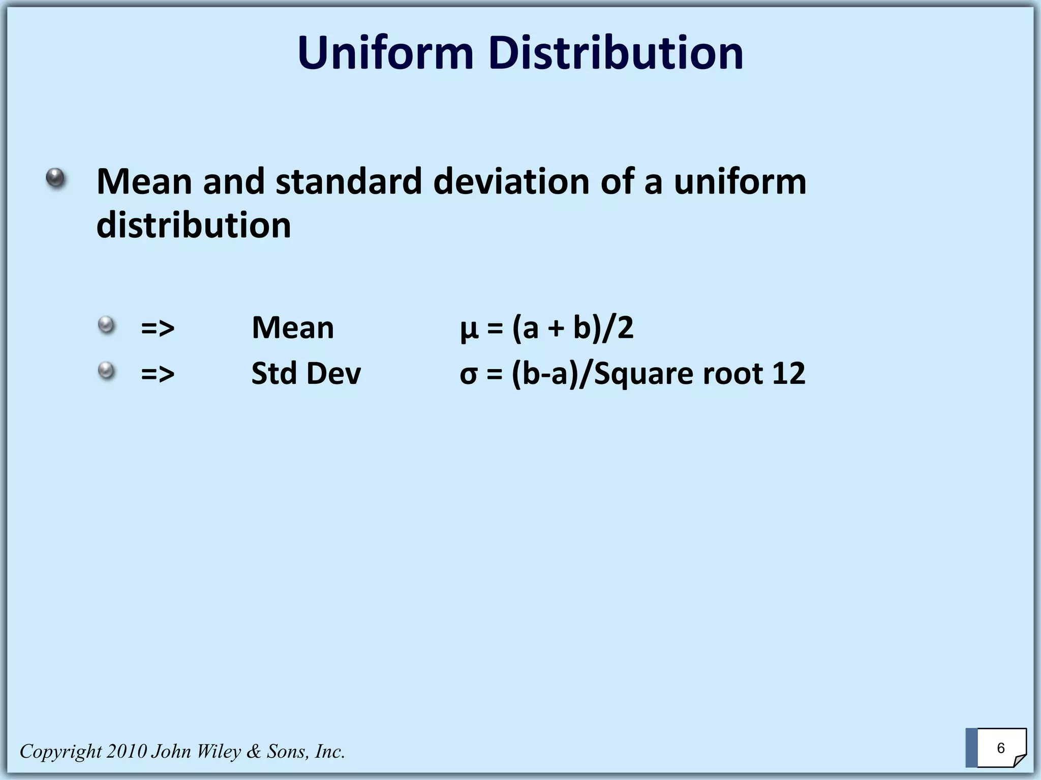
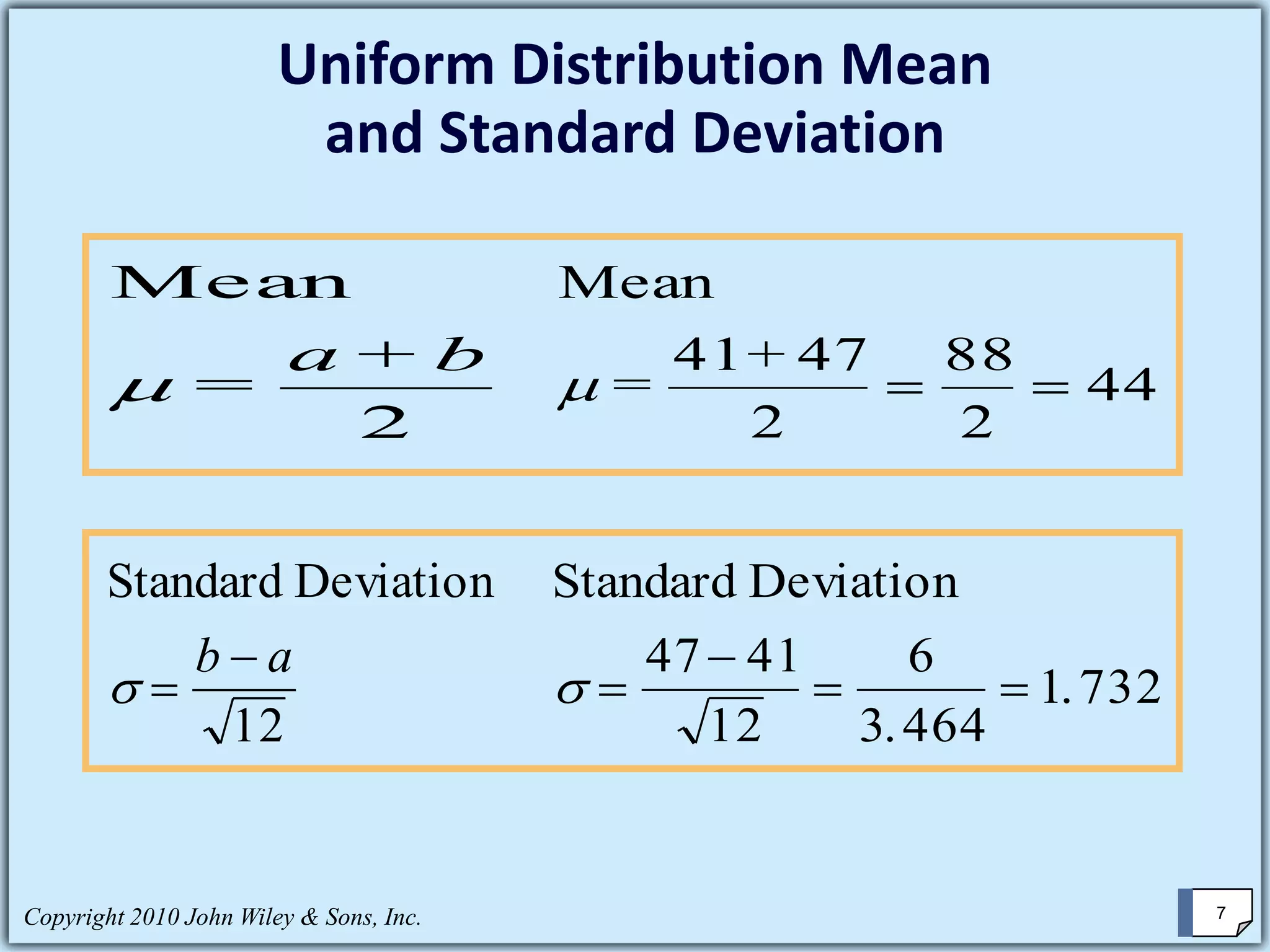
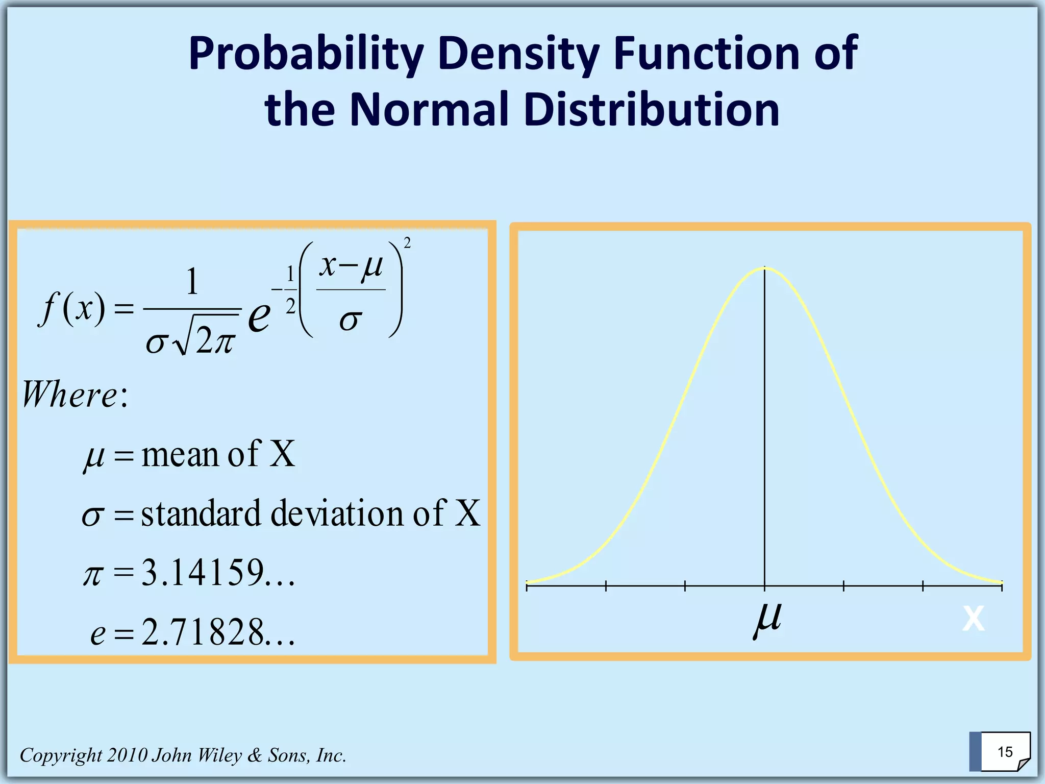
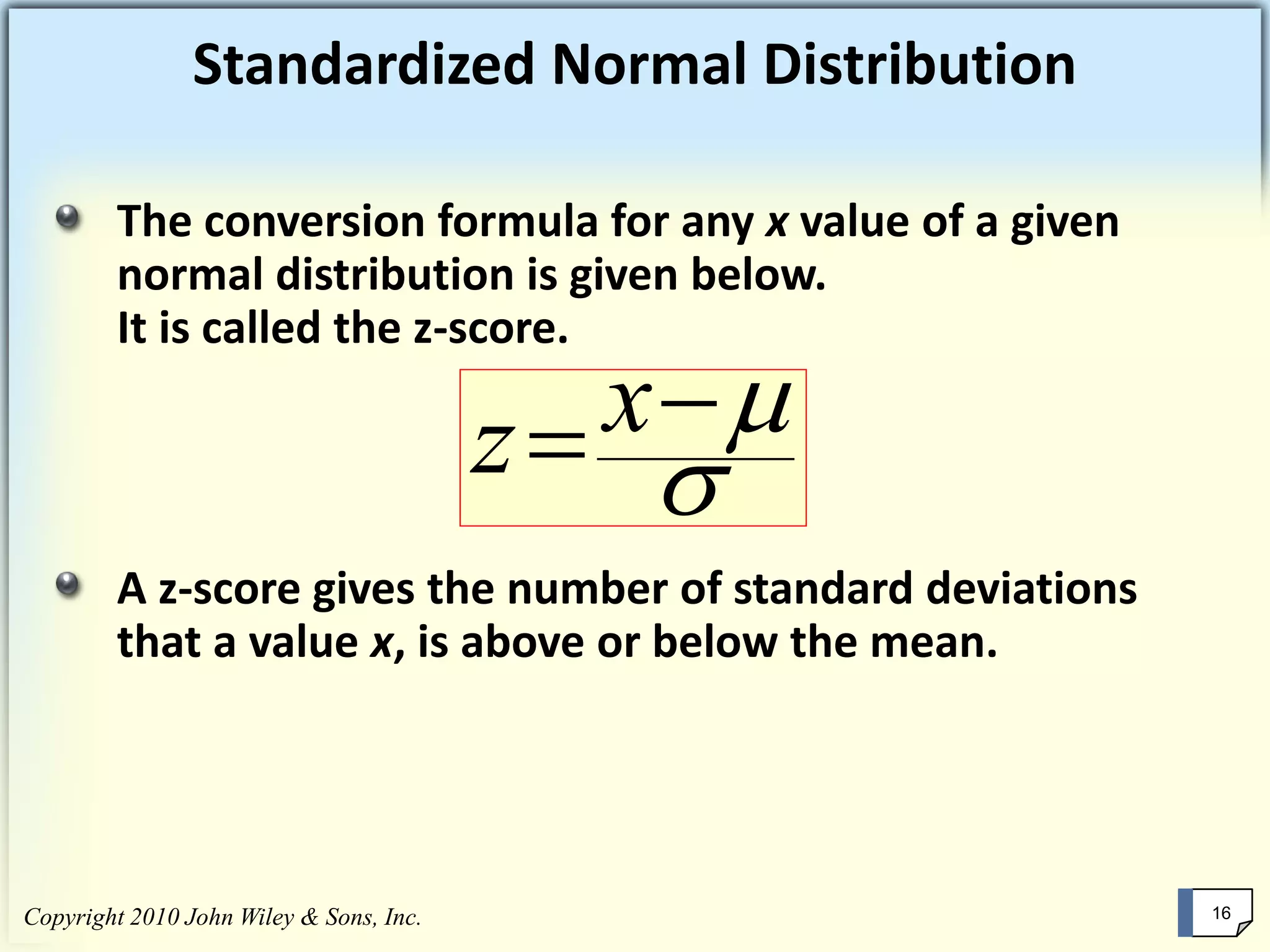
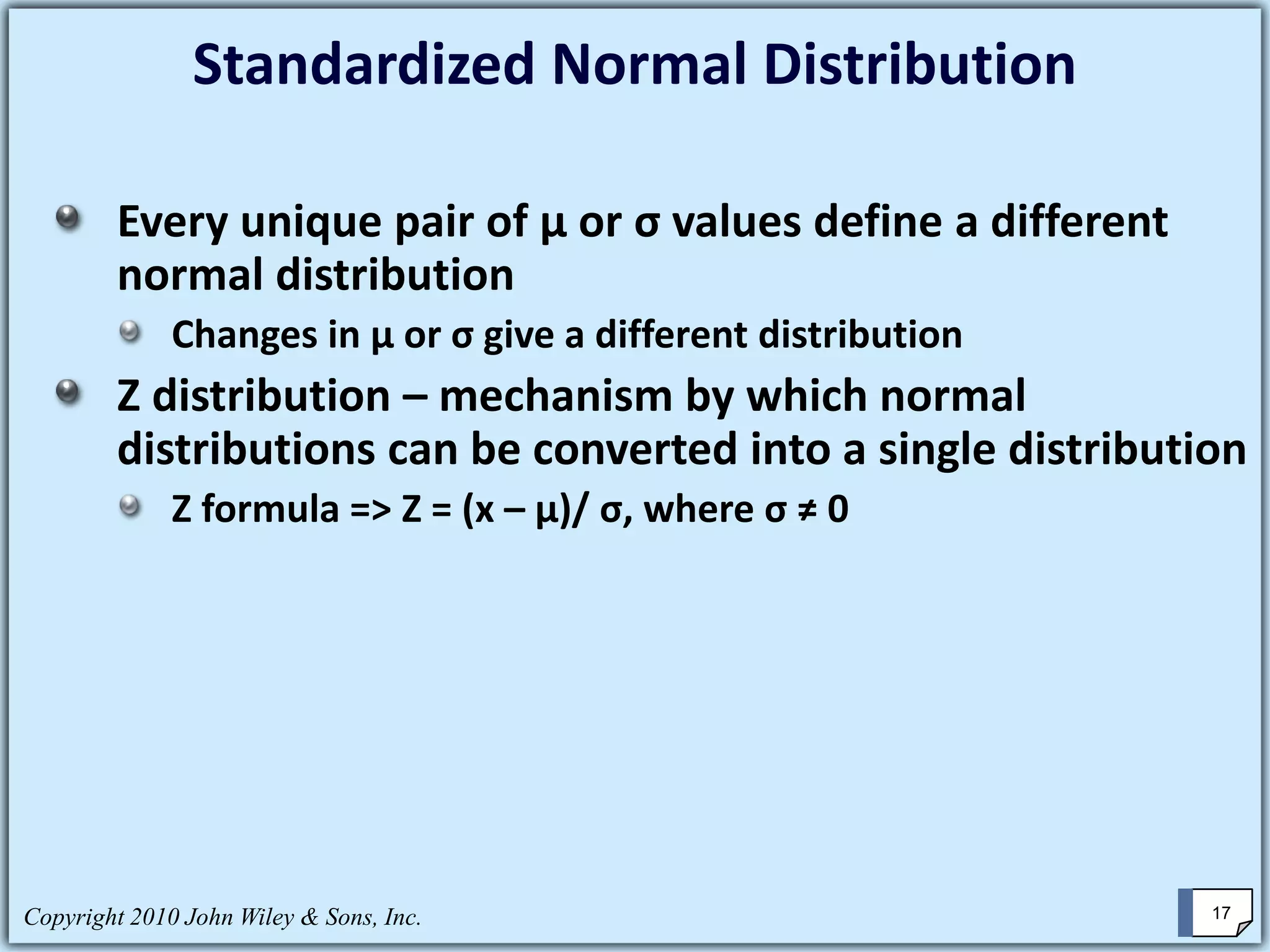
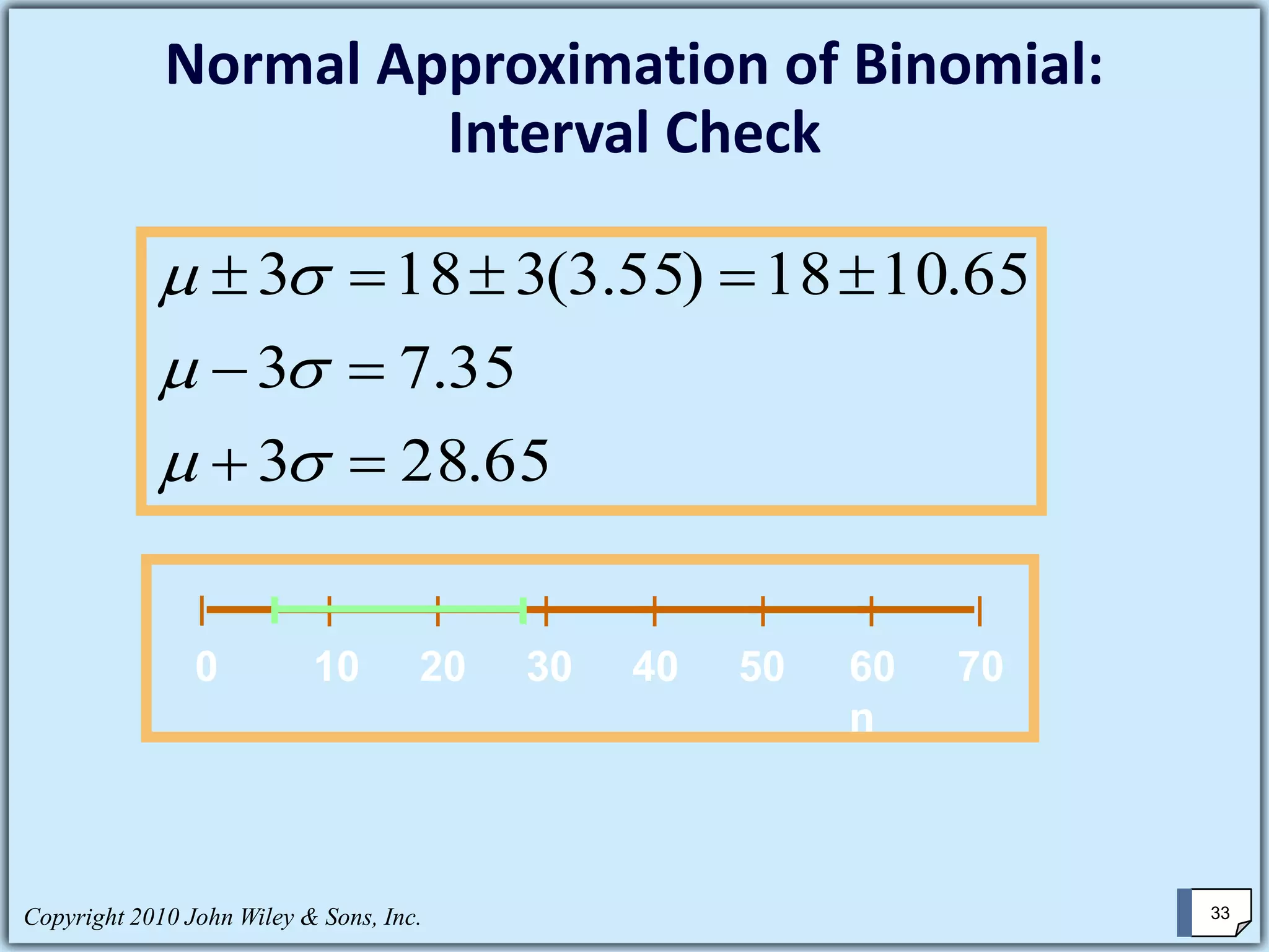
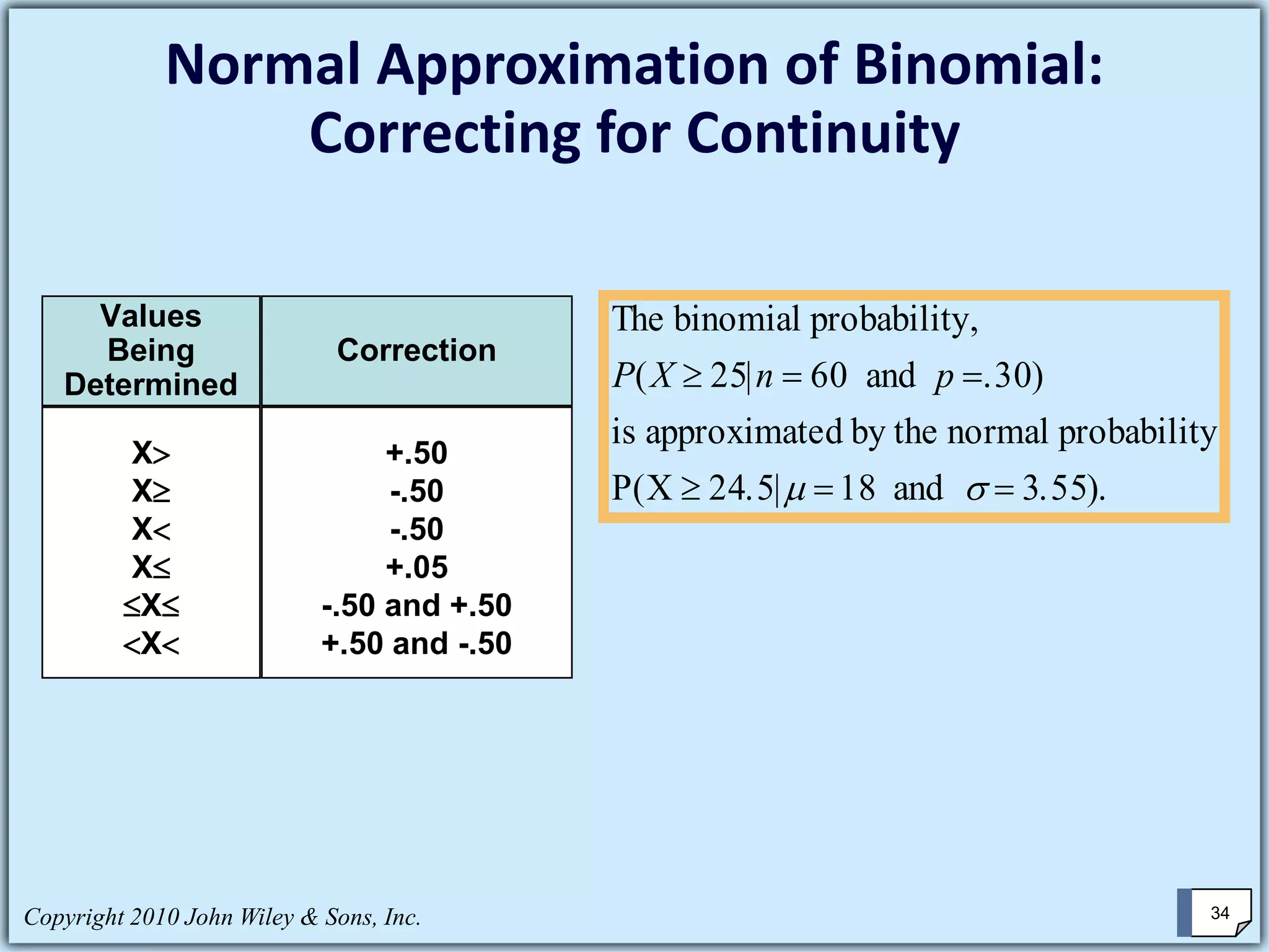
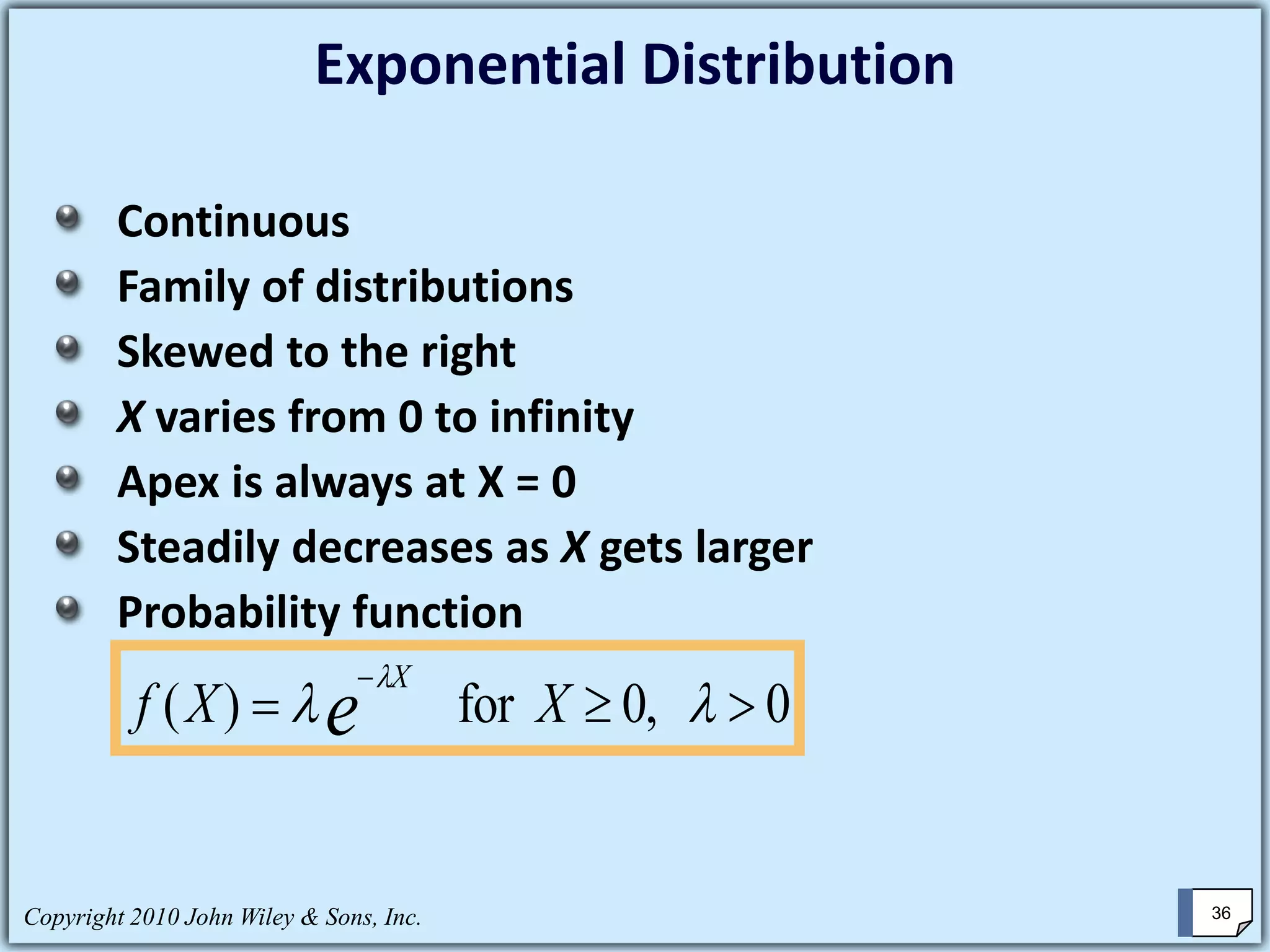
This chapter summary covers key concepts about continuous probability distributions discussed in Chapter 6 of the textbook "Business Statistics, 6th ed." by Ken Black. The chapter objectives are to understand the uniform distribution, appreciate the importance of the normal distribution, and know how to solve normal distribution problems. It discusses the uniform, normal, and exponential distributions. It explains how to calculate probabilities using the normal distribution and z-scores. It also discusses when the normal distribution can be used to approximate the binomial distribution.

1. Business Statistics, 6th ed.
by Ken Black
Chapter 6
Continuous
Probability
Distributions
Copyright 2010 John Wiley & Sons, Inc.

2. Understand concepts of the uniform distribution.
Appreciate the importance of the normal
distribution.
Recognize normal distribution problems, and know
how to solve them.
Decide when to use the normal distribution to
approximate binomial distribution problems, and
know how to work them.
Decide when to use the exponential distribution to
solve problems in business, and know how to work
them.
Copyright 2010 John Wiley & Sons, Inc. 2
Learning Objectives

3. Continuous Distributions
Continuous distributions
Continuous distributions are constructed from continuous
random variables in which values are taken for every point
over a given interval
With continuous distributions, probabilities of outcomes
occurring between particular points are determined by
calculating the area under the curve between these points
Copyright 2010 John Wiley & Sons, Inc. 3

4. Uniform Distribution
The uniform distribution is a relatively simple
continuous distribution in which the same height f(x),
is obtained over a range of values
Copyright 2010 John Wiley & Sons, Inc. 4

5. Uniform Distribution
f x
b a
for a x b
for
( ) =
−
 







1
0 all other values
Area = 1
f x( )
x
1
b a−
a b
Copyright 2010 John Wiley & Sons, Inc. 5

6. Uniform Distribution
Mean and standard deviation of a uniform
distribution
=> Mean μ = (a + b)/2
=> Std Dev σ = (b-a)/Square root 12
Copyright 2010 John Wiley & Sons, Inc. 6

7. Uniform Distribution Mean
and Standard Deviation
Mean
=
+

a b
2
Mean
=
+

41 47
2
88
2
44= =
Standard Deviation
 =
−b a
12
Standard Deviation
 =
−
= =
47 41
12
6
3 464
1 732
.
.
Copyright 2010 John Wiley & Sons, Inc. 7

8. Uniform Distribution of Lot Weights
f x
for x
for
( ) =
−
 







1
47 41
41 47
0 all other values
Area = 1
f x( )
x
6
1
4147
1
=
−
41 47
Copyright 2010 John Wiley & Sons, Inc. 8

9. Uniform Distribution Probability
With discrete distributions, the probability function
yields the value of the probability
For continuous distributions, probabilities are
calculated by determining the area over an interval
of the function
Copyright 2010 John Wiley & Sons, Inc. 9

10. Demonstration Problem 6.1
Suppose the amount of time it takes to assemble a
plastic module ranges from 27 to 39 seconds and that
assembly times are uniformly distributed. Describe the
distribution. What is the probability that a given
assembly will take between 30 and 35 seconds? Fewer
than 30 seconds?
Copyright 2010 John Wiley & Sons, Inc. 10

11. Demonstration Problem 6.1
12
Solution
The height of the distribution is 1 12. The mean time is 33
seconds with a standard deviation of 3.464 seconds.
f (x) = 1/(39 – 27) = 1/12
μ = (a + b)/2 = (39 + 27)/2 = 33
σ = (b – a)/ = (39 – 27)/3.464 = 3.4643
112 =
12
112 = 3.464
Copyright 2010 John Wiley & Sons, Inc. 11

12. Demonstration Problem 6.1
P (30 <x <35) = (35 – 30)/(39 – 27) = 5/12 = .4167
There is a .4167 probability that it will take between 30 and 35
seconds to assemble the module.
P (x < 30) = (30 – 27)/(39 – 27) = 3/12 = .2500
There is a .2500 probability that it will take less than 30 seconds
to assemble the module. Because there is no area less than 27
seconds, P(x < 30) is determined by using only the interval 27 x
30. In a continuous distribution, there is no area at any one point
(only over an interval). Thus the probability x < 30 is the same as
the probability of x … 30.
Copyright 2010 John Wiley & Sons, Inc. 12

13. Properties of the Normal Distribution
Characteristics of the normal distribution:
Continuous distribution - Line does not break
Symmetrical distribution - Each half is a mirror of the other
half
Asymptotic to the horizontal axis - it does not touch the x
axis and goes on forever
Unimodal - means the values mound up in only one portion
of the graph
Area under the curve = 1; total of all probabilities = 1
Copyright 2010 John Wiley & Sons, Inc. 13

14. Probability Density Function of
the Normal Distribution
Normal distribution is characterized by the mean
and the Std Dev
Values of μ and σ produce a normal distribution
Copyright 2010 John Wiley & Sons, Inc. 14

15. Probability Density Function of
the Normal Distribution
...2.71828
...3.14159=
Xofdeviationstandard
Xofmean
:
2
1
)(
2
2
1
=
=
=





 −
=
−
e
Where
x
xf e






 X
Copyright 2010 John Wiley & Sons, Inc. 15

16. Standardized Normal Distribution
The conversion formula for any x value of a given
normal distribution is given below.
It is called the z-score.
A z-score gives the number of standard deviations
that a value x, is above or below the mean.

−= xz
Copyright 2010 John Wiley & Sons, Inc. 16

17. Standardized Normal Distribution
Every unique pair of μ or σ values define a different
normal distribution
Changes in μ or σ give a different distribution
Z distribution – mechanism by which normal
distributions can be converted into a single distribution
Z formula => Z = (x – μ)/ σ, where σ ≠ 0
Copyright 2010 John Wiley & Sons, Inc. 17

18. Standardized Normal Distribution
Z score is the number of Std Dev that a value, x, is
above or below the mean
If x value is less than the mean, the Z score is negative
If x value is greater than mean, the Z score is positive
Copyright 2010 John Wiley & Sons, Inc. 18

19. Z score can be used to find probabilities for any
normal curve problem that has been converted to Z
scores
Z distribution is normal distribution with a mean of 0
and a Std Dev of 1
Standardized Normal Distribution - Continued
Copyright 2010 John Wiley & Sons, Inc. 19

20. Standardized Normal Distribution - Continued
Z distribution probability values are given in table A5
Table A5 gives the total area under the Z curve
between 0 and any point on the positive Z axis
Since the curve is symmetric, the area under the curve
between Z and 0 is the same whether the Z curve is
positive or negative
Copyright 2010 John Wiley & Sons, Inc. 20

21. A normal distribution with
a mean of zero, and
a standard deviation of one
Z Formula
standardizes any normal distribution
Z Score
computed by the Z Formula
the number of standard
deviations which a value
is away from the mean

−
=
X
Z
 = 1
 = 0
Standardized Normal Distribution - Continued
Copyright 2010 John Wiley & Sons, Inc. 21

22. Standardized Normal Distribution - Continued
If x is normally distributed with a mean of  and a
standard deviation of , then the z-score will also be
normally distributed with a mean of 0 and a standard
deviation of 1.
Tables have been generated for standard normal
distribution which enable you to determine
probabilities for normal variables.
The tables are set to give the probabilities between
z = 0 and some other z value, z0 say, which is depicted
on the next slide.
Copyright 2010 John Wiley & Sons, Inc. 22

23. Z Table
Second Decimal Place in Z
Z 0.00 0.01 0.02 0.03 0.04 0.05 0.06 0.07 0.08 0.09
0.00 0.0000 0.0040 0.0080 0.0120 0.0160 0.0199 0.0239 0.0279 0.0319 0.0359
0.10 0.0398 0.0438 0.0478 0.0517 0.0557 0.0596 0.0636 0.0675 0.0714 0.0753
0.20 0.0793 0.0832 0.0871 0.0910 0.0948 0.0987 0.1026 0.1064 0.1103 0.1141
0.30 0.1179 0.1217 0.1255 0.1293 0.1331 0.1368 0.1406 0.1443 0.1480 0.1517
0.90 0.3159 0.3186 0.3212 0.3238 0.3264 0.3289 0.3315 0.3340 0.3365 0.3389
1.00 0.3413 0.3438 0.3461 0.3485 0.3508 0.3531 0.3554 0.3577 0.3599 0.3621
1.10 0.3643 0.3665 0.3686 0.3708 0.3729 0.3749 0.3770 0.3790 0.3810 0.3830
1.20 0.3849 0.3869 0.3888 0.3907 0.3925 0.3944 0.3962 0.3980 0.3997 0.4015
2.00 0.4772 0.4778 0.4783 0.4788 0.4793 0.4798 0.4803 0.4808 0.4812 0.4817
3.00 0.4987 0.4987 0.4987 0.4988 0.4988 0.4989 0.4989 0.4989 0.4990 0.4990
3.40 0.4997 0.4997 0.4997 0.4997 0.4997 0.4997 0.4997 0.4997 0.4997 0.4998
3.50 0.4998 0.4998 0.4998 0.4998 0.4998 0.4998 0.4998 0.4998 0.4998 0.4998
Copyright 2010 John Wiley & Sons, Inc. 23

24. Table Lookup of a Standard
Normal Probability
-3 -2 -1 0 1 2 3
P Z( ) .0 1 0 3413  =
Z 0.00 0.01 0.02
0.00 0.0000 0.0040 0.0080
0.10 0.0398 0.0438 0.0478
0.20 0.0793 0.0832 0.0871
1.00 0.3413 0.3438 0.3461
1.10 0.3643 0.3665 0.3686
1.20 0.3849 0.3869 0.3888
Copyright 2010 John Wiley & Sons, Inc. 24

25. Applying the Z Formula
X is normally distributed with = 485, and =105 
P X P Z( ) ( . ) .485 600 0 1 10 3643  =   =
For X = 485,
Z =
X-

=
−
=
485 485
105
0
10.1
105
485600-X
=Z
600,=XFor
=
−
=


Z 0.00 0.01 0.02
0.00 0.0000 0.0040 0.0080
0.10 0.0398 0.0438 0.0478
1.00 0.3413 0.3438 0.3461
1.10 0.3643 0.3665 0.3686
1.20 0.3849 0.3869 0.3888
Copyright 2010 John Wiley & Sons, Inc. 25

26. Applying the Z Formula
X is normally distributed with = 485, and =105 
P X P Z( ) ( . ) .485 600 0 1 10 3643  =   =
For X = 485,
Z =
X-

=
−
=
485 485
105
0
For X = 600,
Z =
X-

=
−
=
600 485
105
1 10.
Z 0.00 0.01 0.02
0.00 0.0000 0.0040 0.0080
0.10 0.0398 0.0438 0.0478
1.00 0.3413 0.3438 0.3461
1.10 0.3643 0.3665 0.3686
1.20 0.3849 0.3869 0.3888
Copyright 2010 John Wiley & Sons, Inc. 26

27. Applying the Z Formula
7123.)56.0()550(
100=and494,=withddistributenormallyisX
== ZPXP

56.0
100
494550-X
=Z
550=XFor
=
−
=


0.5 + 0.2123 = 0.7123
Copyright 2010 John Wiley & Sons, Inc. 27

28. Applying the Z Formula
0197.)06.2()700(
100=and494,=withddistributenormallyisX
== ZPXP

06.2
100
494700-X
=Z
700=XFor
=
−
=


0.5 – 0.4803 = 0.0197
Copyright 2010 John Wiley & Sons, Inc. 28

29. Applying the Z Formula
94.1
100
494300-X
=Z
300=XFor
−=
−
=


8292.)06.194.1()600300(
100=and494,=withddistributenormallyisX
=−= ZPXP

0.4738+ 0.3554 = 0.8292
06.1
100
494600-X
=Z
600=XFor
=
−
=


Copyright 2010 John Wiley & Sons, Inc. 29

30. Normal Approximation of the
Binomial Distribution
For certain types of binomial distributions, the
normal distribution can be used to approximate the
probabilities
At large sample sizes, binomial distributions approach the
normal distribution in shape regardless of the value of p
The normal distribution is a good approximate for binomial
distribution problems for large values of n
Copyright 2010 John Wiley & Sons, Inc. 30

31. Demonstration Problem 6.9
These types of problems can be solved quite easily
with the appropriate technology. The output shows
the MINITAB solution.
Copyright 2010 John Wiley & Sons, Inc. 31

32. Normal Approximation of Binomial:
Parameter Conversion
Conversion equations
Conversion example:


= 
=  
n p
n p q
Given that X has a binomial distribution, find
andP X n p
n p
n p q
( | . ).
( )(. )
( )(. )(. ) .
 = =
=  = =
=   = =
25 60 30
60 30 18
60 30 70 3 55


Copyright 2010 John Wiley & Sons, Inc. 32

33. 65.283
35.73
65.1018)55.3(3183
=+
=−
==



0 10 20 30 40 50 60
n
70
Normal Approximation of Binomial:
Interval Check
Copyright 2010 John Wiley & Sons, Inc. 33

34. Normal Approximation of Binomial:
Correcting for Continuity
Values
Being
Determined
Correction
X
X
X
X
X
X
+.50
-.50
-.50
+.05
-.50 and +.50
+.50 and -.50
The binomial probability,
and
is approximated by the normal probability
P(X 24.5| and
P X n p( | . )
. ).
 = =
 = =
25 60 30
18 3 55 
Copyright 2010 John Wiley & Sons, Inc. 34

35. 25
26
27
28
29
30
31
32
33
Total
0.0167
0.0096
0.0052
0.0026
0.0012
0.0005
0.0002
0.0001
0.0000
0.0361
X P(X)
( )
The normal approximation,
P(X 24.5| and = =
= 
−





= 
= −  
= −
=
 18 355
24 5 18
355
183
5 0 183
5 4664
0336
. )
.
.
( . )
. .
. .
.
P Z
P Z
P Z
Normal Approximation of Binomial:
Computations
Copyright 2010 John Wiley & Sons, Inc. 35

36. f X X
X
e( ) ,=  
−
 

for 0 0
Exponential Distribution
Continuous
Family of distributions
Skewed to the right
X varies from 0 to infinity
Apex is always at X = 0
Steadily decreases as X gets larger
Probability function
Copyright 2010 John Wiley & Sons, Inc. 36

37. Different Exponential Distributions
Copyright 2010 John Wiley & Sons, Inc. 37

38. 0.0
0.2
0.4
0.6
0.8
1.0
1.2
0 1 2 3 4 5
 =  ( )
( )
P X X
X
P X
e
e
 =
−
 = =
−
=
0
0
2 12
12 2
0907

| .
( . )( )
.
Exponential Distribution: Probability
Computation
Copyright 2010 John Wiley & Sons, Inc. 38