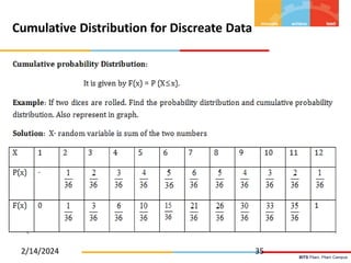
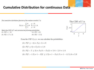
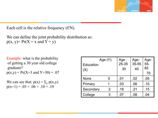
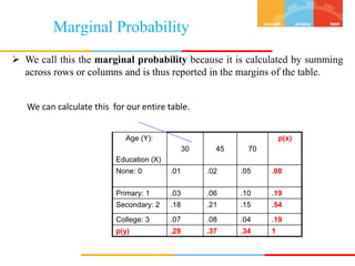
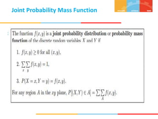
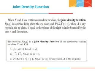
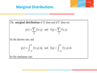
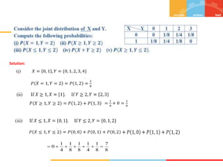
The document discusses random variables and their probability distributions. It defines discrete and continuous random variables and their key characteristics. Discrete random variables can take on countable values while continuous can take any value in an interval. Probability distributions describe the probabilities of a random variable taking on different values. The mean and variance are discussed as measures of central tendency and variability. Joint probability distributions are introduced for two random variables. Examples and homework problems are also provided.

1. BITS Pilani
Pilani Campus
Introduction
to Statistical Methods
ISM Team

2. BITS Pilani
Pilani Campus
M.Tech. (AIML)
Session-5 (Random Variables)
Team ISM

3. IMP Note to Self

5. Random variables –
Discrete & continuous Expectation of a random variable,
mean and variance of a random variable –
Single random random variable &
Joint distributions
Session-5 Agenda

6. Random Variables
 A random variable is a variable that assumes numerical values
associated with the random outcome of an experiment, where
one (and only one) numerical value is assigned to each sample
point.
 In mathematical language, a random variable is a function
whose domain is the sample space and whose range is the set
of real numbers.

7.  A random variable can be classified as being either discrete
or continuous depending on the numerical values it assumes.
 A discrete random variable may assume either finite or
countably infinite number of values
 A continuous random variable may assume any numerical
value in an interval or collection of intervals.
 Continuous random variables are generated in experiments
where things are “measured’ as opposed to “counted”.
 Experimental outcomes based on measurement of time,
distance, weight, volume etc. generate continuous RV.
Random Variables

8. Types of random Variables
 A discrete random variable can assume a countable
number of values.
o Number of steps to the top of the Eiffel Tower*
 A continuous random variable can assume any
value along a given interval of a number line.
o The time a tourist stays at the top once s/he gets there
8

9.  Discrete random variables
o Number of sales
o Number of calls
o Shares of stock
o People in line
o Mistakes per page
Two Types of Random Variables
 Continuous random variables
o Length
o Depth
o Volume
o Time
o Weight

10.  The probability distribution for a random variable describes how
probabilities are distributed over the values of the random variable.
 The probability distribution is defined by a probability function, denoted
by f(x), which provides the probability for each value of the random
variable.
The required conditions for a discrete probability function are:
f(x) > 0
f(x) = 1
 We can describe a discrete probability distribution with a table, graph, or
equation.
 Advantage: once the probability distribution is known, it is relatively easy
to determine the probability of a variety of events that may be of interest
to the decision maker.
Discrete Probability Distributions

11. Probability Distributions for
Discrete Random Variables
• Say a random variable x
follows this pattern: p(x) =
(.3)(.7)x-1 for x >0.
– This table gives the
probabilities (rounded to
two digits) for x between 1
and 10.
x P(x)
1 .30
2 .21
3 .15
4 .11
5 .07
6 .05
7 .04
8 .02
9 .02
10 .01
11
McClave, Statistics, 11th ed. Chapter 4:
Discrete Random Variables

12.  The expected value, or mean, of a random variable is a measure of
its central location.
o The mean or Expected value of a discrete random variable:
E(x) =  = xf(x)
 The variance summarizes the variability in the values of a random
variable.
o Variance of a discrete random variable:
Var(x) =  2 = (x - )2f(x)
 The standard deviation, , is defined as the positive square root of the variance.
Expected Value and Variance

13. Rules of Expected Value
 Multiplying RV by a constant a, E(aX) = a.E(X)
 Adding a constant b, E(X+b) = E(X) + b
 Therefore, E(aX + b) = ?

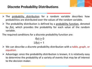
14. 2 2 2
[( ) ] ( ) ( ).
E x x p x
  
   

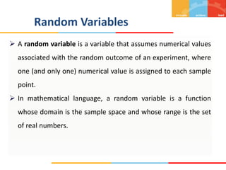
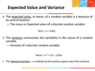
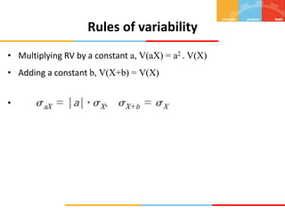
Variability of Discrete Random Variables
 The variance of a discrete random variable x is
 The standard deviation of a discrete random variable x is
2 2 2
[( ) ] ( ) ( ).
E x x p x
  
   


15. Rules of variability
• Multiplying RV by a constant a, V(aX) = a2 . V(X)
• Adding a constant b, V(X+b) = V(X)
•

16. At a shooting range, a shooter is able to hit a target in either 1, 2
or 3 shots. Let x be a random variable indicating the number of
shots fired to hit the target. The following probability function
was proposed.
f(x) = x/6
Is this probability function valid?
Identify the r.v to be discrete or continuous?
Example
EXPERIMENT Random Variable (x)
Audit 50 tax returns Number of returns that contains error
Operate a restaurant for one day Number of customers
Observe an employee’s work No. of productive hours in an 8-hour workday

17.  The discrete uniform probability distribution is the simplest
example of a discrete probability distribution given by a formula.
o The discrete uniform probability function is
f(x) = 1/n
where:
n = the number of values the random variable may assume
Note that the values of the random variable are equally likely.
Discrete Uniform Probability Distribution

18. BITS Pilani, Pilani Campus
Random
variable
Discrete
Probability mass
function(pmf)
f(x)
Cumulative
distribution
function
F(x)
Continuous
Probability Density
function(pdf)
f(x)
Cumulative
distribution
function
F(x)

20.  A continuous random variable can assume any value in an interval
on the real line or in a collection of intervals.
 It is not possible to talk about the probability of the random
variable assuming a particular value.
 Instead, we talk about the probability of the random variable
assuming a value within a given interval.
 The probability of the random variable assuming a value within
some given interval from x1 to x2 is defined to be the area under
the graph of the probability density function between x1 and x2.
Continuous Probability Distributions

21. BITS Pilani, Pilani Campus
Continuous Random Variables
Example:
o Height of students in a class
o Amount of ice tea in a glass
o Change in temperature throughout a day
o Price of a car in next year

22. BITS Pilani, Pilani Campus
Continuous Random Variables

23. BITS Pilani, Pilani Campus
Continuous Random Variables

24. BITS Pilani, Pilani Campus
Continuous Random Variables

25. BITS Pilani, Pilani Campus
Integration Formulas

26. BITS Pilani, Pilani Campus
2/14/2024 26
Continuous Random Variables

27. BITS Pilani, Pilani Campus

28. BITS Pilani, Pilani Campus

29. BITS Pilani, Pilani Campus
2/14/2024 29

30. BITS Pilani, Pilani Campus
Home Assignments
Example:1
Example:2

31. BITS Pilani, Pilani Campus
2/14/2024 31
Example:3

32. BITS Pilani, Pilani Campus
Example:4
Example:5

33. BITS Pilani, Pilani Campus
2/14/2024 33
Example:6

34. BITS Pilani, Pilani Campus
2/14/2024 34
Example:7

35. BITS Pilani, Pilani Campus
2/14/2024 35
Cumulative Distribution for Discreate Data

36. BITS Pilani, Pilani Campus
Cumulative Distribution for continuous Data

38. So far we have been talking about the probability of a single variable, or a variable
conditional on another.
We often want to determine the joint probability of two variables, such as X and Y.
Suppose we are able to determine the following information for education (X)
and age (Y) for all Indian citizens based on the census.
Age (Y):
Education
(X)
Age : 25-35
30
Age: 35-55
45
Age: 55-85
70
None 0 .01 .02 .05
Primary 1 .03 .06 .10
Secondary 2 .18 .21 .15
College 3 .07 .08 .04

39. Example: what is the probability
of getting a 30 year old college
graduate?
p(x,y) = Pr(X=3 and Y=30) = .07
We can see that: p(x) = y p(x,y)
p(x=1) = .03 + .06 + .10 = .19
Each cell is the relative frequency (f/N).
We can define the joint probability distribution as:
p(x, y)= Pr(X = x and Y = y)
Age (Y):
Education
(X)
Age :
25-35
30
Age:
35-55
45
Age:
55-
85
70
None 0 .01 .02 .05
Primary 1 .03 .06 .10
Secondary 2 .18 .21 .15
College 3 .07 .08 .04

40. Marginal Probability
 We call this the marginal probability because it is calculated by summing
across rows or columns and is thus reported in the margins of the table.
We can calculate this for our entire table.
Age (Y):
Education (X)
30 45 70
p(x)
None: 0 .01 .02 .05 .08
Primary: 1 .03 .06 .10 .19
Secondary: 2 .18 .21 .15 .54
College: 3 .07 .08 .04 .19
p(y) .29 .37 .34 1

41. If X and Y are discrete random variables, the joint probability distribution of X
and Y is a description of the set of points (x,y) in the range of (X,Y) along with
the probability of each point.
The joint probability distribution of two discrete random variables is sometimes
referred to as the bivariate probability distribution or bivariate
distribution.
Thus we can describe the joint probability distribution of two discrete random
variables is through a joint probability mass function
f(x,y)=P(X=x,Y=y)

42. Joint Probability Mass Function

43. Joint Density Function

44. Marginal Distributions

45. 8
7
8
1
4
1
8
1
8
1
4
1
0 






Solution:

46. Cont.

47. Problem:
 Two ballpoint pens are selected at random form a box that contains blue
pens, 2 red pens and 3 green pens. If X is the number of blue pens selected
and Y is the number of red pens selected, find the joint probability
function f(x,y)
 Solution:
The possible pairs of values (x,y) are (0,0),(0,1),(1,0),(1,1),(0,2),(2,0)
The joint probability distribution can be represented by the formula

48. f(x,y) X Rows
Total
0 1 2
y
0 3/28 9/28 3/28 15/28
1 3/14 3/14 0 3/7
2 1/28 0 0 1/28
Columns Total 5/14 15/28 3/28 1
Joint distribution

49. Solution:
Example

50. Homework Assignment

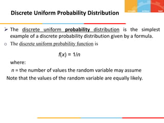
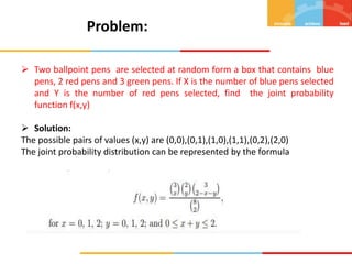
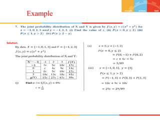
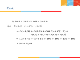
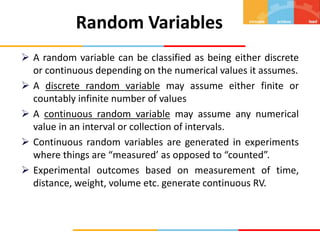
51. A candy company distributed boxes of chocolates with a mixture of creams, toffees,
and nuts coated in both light and dark chocolate. For a randomly selected box, let X
and Y, respectively, be the proportions of the light and dark chocolates that are creams
and suppose that the joint density function is
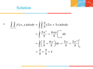
a) Verify whether
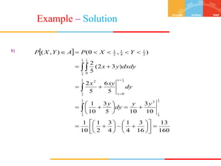
b) Find P[(X,Y)  A], where A is the region {(x,y) | 0<x<½,¼<y<½}
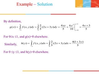
c) Find g(x) and h(y) for the joint density function.


 





elsewhere
,
0
1
0
,
1
0
),
3
2
(
)
,
( 5
2
y
x
y
x
y
x
f
 






 1
y)dxdy
f(x,
Home work Assignment:

52. 1
5
3
5
2
5
3
5
2
5
6
5
2
5
6
5
2
)
3
2
(
5
2
)
,
(
1
0
2
1
0
1
0
1
0
2
1
0
1
0



















 
 








y
y
dy
y
dy
xy
x
dxdy
y
x
dxdy
y
x
f
x
x
a)
Solution

53.  
160
13
16
3
4
1
4
3
2
1
10
1
10
3
10
5
3
10
1
5
6
5
2
)
3
2
(
5
2
)
,
0
(
)
,
(
2
1
4
1
2
1
4
1
2
1
4
1
2
1
2
1
4
1
2
1
2
0
2
0
2
1
4
1
2
1













































 


y
y
dy
y
dy
xy
x
dxdy
y
x
Y
X
P
A
Y
X
P
x
x
b)
Example – Solution

54. 5
3
4
10
6
5
4
)
3
2
(
5
2
)
,
(
)
(
1
0
2
1
0














x
y
xy
dy
y
x
dy
y
x
f
x
g
y
y
5
)
3
1
(
4
)
3
2
(
5
2
)
,
(
)
(
1
0
y
dx
y
x
dx
y
x
f
y
h




 




By definition,
For 0x 1, and g(x)=0 elsewhere.
Similarly,
For 0 y 1, and h(y)=0 elsewhere.
Example – Solution

55. Problem:
Find ‘K’ if the joint probability density function of a bivariate
random variable (X,Y) is given by


 




otherwise
x
if
y
x
K
y
x
f
0
4
0
)
1
)(
1
(
)
,
(

56. Solution:
Example

57. Cont.

58. IMP Note to Self

59. Thank You !