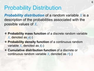
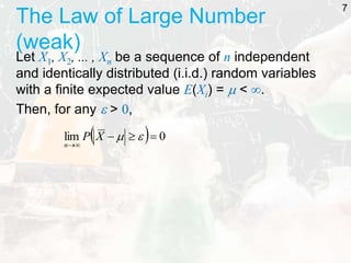
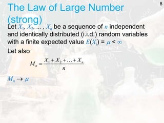
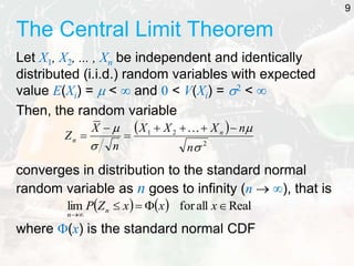
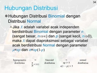
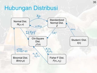
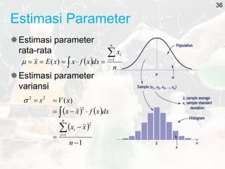
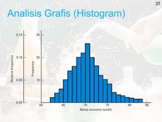
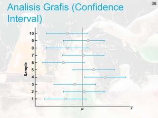
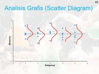
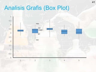
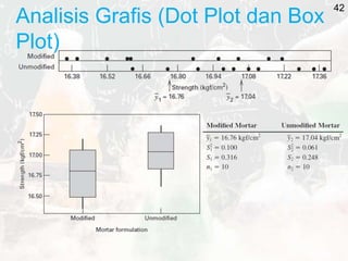
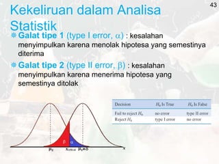
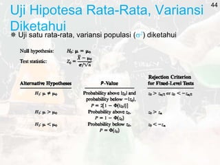
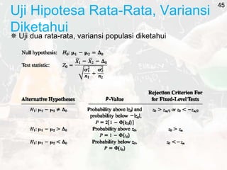
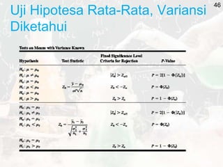
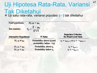
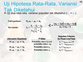
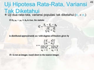
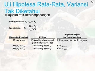
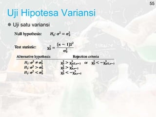
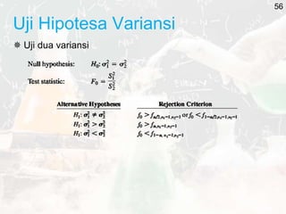
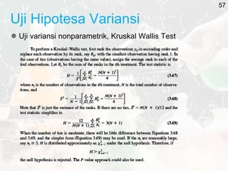
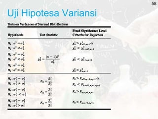
The document outlines key statistical concepts including probability, random variables, and various probability distributions such as normal, binomial, and chi-square distributions. It discusses foundational theorems like the Law of Large Numbers and the Central Limit Theorem, as well as hypothesis testing methods and potential errors in statistical analysis. Additionally, it highlights graphical analysis techniques and parameter estimation related to these statistical methods.

1. Statistics for
Experiments
ARIF RAHMAN
1

2. Statistics Prerequisite
2

3. Random Experiments
Sample space is the set of all possible outcomes
of a random experiment.
Sample point is each outcome in a sample
space.
Outcome is an element of a sample space.
Event is a subset of a sample space.
Probability is a number that is assigned to each
member of a collection of events from a random
experiment.
3

4. Axioms of Probability
If S is the sample space and E is any event in a
random experiment, probability satisfies the
following properties:
(1) P(S) = 1
(2) 0 < P(E) < 1
(3) P(E1  E2) = P(E1) + P(E2) - P(E1  E2)
(4) P(E1 | E2) = P(E1  E2) / P(E2)
4

5. Random Variable
Random variable is a function that assigns a real
number to each outcome in the sample space of a
random experiment.
Random variable is denoted by an uppercase letter, such as X.
After an experiment is conducted, the measured value of the
random variable is denoted by a lowercase letter, such as x.
 A discrete random variable is a random variable with an interval
(either finite or infinite) of natural number (or non-negative integers), N,
for its range.
 A continuous random variable is a random variable with an interval
(either finite or infinite) of real numbers, R, for its range.
5

6. Probability Distribution
Probability distribution of a random variable X is a
description of the probabilities associated with the
possible values of X.
 Probability mass function of a discrete random variable
X, denoted as p(x)
 Probability density function of a continuous random
variable X, denoted as f(x)
 Cumulative distribution function of a discrete or
continuous random variable X, denoted as F(x)
6

7. The Law of Large Number
(weak)
Let X1, X2, ... , Xn be a sequence of n independent
and identically distributed (i.i.d.) random variables
with a finite expected value E(Xi) =  < .
Then, for any  > 0,
7
  0
lim 






X
P
n

8. The Law of Large Number
(strong)
Let X1, X2, ... , Xn be a sequence of n independent
and identically distributed (i.i.d.) random variables
with a finite expected value E(Xi) =  < 
Let also
Mn  
8
n
X
X
X
M n
n





2
1

9. The Central Limit Theorem
Let X1, X2, ... , Xn be independent and identically
distributed (i.i.d.) random variables with expected
value E(Xi) =  <  and 0 < V(Xi) = 2 < 
Then, the random variable
converges in distribution to the standard normal
random variable as n goes to infinity (n  ), that is
where (x) is the standard normal CDF
9
 
2
2
1




n
n
X
X
X
n
X
Z n
n








    Real
all
for
lim 





x
x
x
Z
P n
n

10. Cochran’s Theorem
Let Zi be normally and independently distributed
NID(0,1) with parameter  = 0 dan  = 1,
for i = 1,2,...,. and
where s <  and Qi has i degrees of freedom (i =
1,2,...,s). Maka Q1, Q2,..., Qs are independent
chi-square variables with 1, 2,..., s degrees of
freedom, respectively, if and only if
s
i
i Q
Q
Q
Z 





...
2
1
1
2

s



 


 ...
2
1
10

11. Normal Distribution Uniform Distribution Negative-Exponential 11

12. Normal
Distribution
Uniform
Distribution
Negative
Exponential
12

13. Normal Distribution
Normal distribution or Gaussian distribution is a
probability distribution function of continuous
random variable X that has a symmetrical bell-
shaped curve. Most of the observations cluster
around the central peak and the probabilities for
values further away from the mean taper off equally
in both directions. Extreme values in both tails of the
distribution are similarly unlikely.
Random variable is an interval infinite of real
number from negative infinite - to infinite (), X{-
<x<}.
13

14. Normal Distribution
Penerapan Distribusi Normal antara lain
untuk menunjukkan sebaran data hasil
pengukuran ilmiah baik observasi ataupun
eksperimen, sebaran kesalahan, sebaran
rata-rata data subgrup, sebaran data yang
sangat banyak (Law of Large Number dan
Central Limit Theorem).
14

15. Normal Distribution
 Parameter   (mean) dan  (standard deviation)
 Probability Density Function, f(x)
 Cummulative Distribution Function, F(x)
2
)
2
/(
)
(
.
2
)
(
2
2







x
e
x
f



x
di
i
f
x
F )
(
)
(
15

16. Normal Distribution
Denoted by N(x;,)
Parameter   dan 
Mean
Variance

 
2
2

 
16

17. Standardized Normal Distribution
Standardized Normal Distribution is
normal distribution with parameter  = 0 and
 = 1
Standardized Normal Distribution is also
called by Z Distribution.
17

18. Standardized Normal Distribution
 Parameter   (mean) dan  (standard deviation)
 Probability Density Function, f(x)
 Cummulative Distribution Function, F(x)

2
)
(
2
/
2
x
e
x
f





x
di
i
f
x
F )
(
)
(
18

19. Distribusi Standardized Normal
Denoted by Z(x)
Parameter  =0 dan =1
Mean
Variance
0


1
2


19

20. Student’s t Distribution
Distribusi Student’s t adalah sebaran
variabel acak yang merupakan model
gabungan variabel acak X berdistribusi
Standard Normal yang mempunyai
parameter =0 dan =1 dengan variabel
acak Y berdistribusi Chi square dengan
derajat bebas sebesar  yang mempunyai
parameter =/2 dan =2.









Y
X
20

21. Student’s t Distribution
 Parameter   (degree of freedom)
 Probability Density Function, f(x)
 Cummulative Distribution Function, F(x)
 
 
 
2
1
2
2
2
1
1
)
(





















x
x
f



x
di
i
f
x
F )
(
)
(
21

22. Student’s t Distribution
Denoted by Student(x;) atau t
Parameter   (degree of freedom)
Mean
Variance
0


2
2





22

23. Chi-Square Distribution
 Parameter   (degree of freedom)
 Probability Density Function, f(x)
 Cummulative Distribution Function, F(x)








 0
)
(
0
0
)
(
0
x
di
i
f
x
x
F
x











other
x
e
x
x
f
x
0
0
)
(
2
)
( 2
2
/
1
)
2
/
(
2
/



  )
1
(
1
)
(
0
1





 





 
dx
e
x x
23

24. Chi-Square Distribution
Denoted by CHISQR(x;) atau 2
Parameter   (degree of freedom)
Mean
Variance

 

 2
2

24

25. Fisher F Distribution
 Parameter  1, 2 (degree of freedom)
 Probability Density Function, f(x)
 Cummulative Distribution Function, F(x)








 0
)
(
0
0
)
(
0
x
di
i
f
x
x
F
x
 
 












other
x
x
x
x
x
f
0
0
)
,
(
)
(
2
2
2
1
2
1
2
1
2
2
1
1










   
 





 








 


1
0
1
1
)
1
(
)
,
( dx
x
x
25

26. Fisher F Distribution
Denoted by F(x;1,2)
Parameter  1, 2 (degree of freedom)
Mean
Variance
2
2
2





 
   
4
2
2
2
2
2
2
1
2
1
2
2
2












26

27. Binomial Distribution
 Parameter  p (probability of success) dan n (number of
trials)
 Probability Mass Function, p(x)
 Cummulative Distribution Function, F(x)

















other
n
x
p
p
x
n
x
p
x
n
x
0
,...,
1
,
0
)
1
(
)
(










0
)
(
0
0
)
(
0
x
i
p
x
x
F
x
i
27

28. Binomial Distribution
Denoted by BIN(x;n,p)
Parameter  p dan n
Mean
Variance
p
n.


)
1
(
.
2
p
p
n 


28

29. Probability Distribution Function
29

30. Hubungan Distribusi
Hubungan Distribusi Standard
(Standardized) Normal dengan Distribusi
Normal
Jika X adalah variabel acak independen
berdistribusi Normal (,), maka adalah
variabel acak berdistribusi Standard Normal




X
Z
30

31. Hubungan Distribusi
Hubungan Distribusi Student’s t dengan
Distribusi Standard (Standardized) Normal
Jika X adalah variabel acak independen
berdistribusi Normal (=0,=1), dan Y adalah
variabel acak independen berdistribusi Chi
square dengan derajat kebebasan sebesar 
maka adalah variabel acak berdistribusi
Student’s t yang mempunyai parameter =/2
dan =2









Y
X
31

32. Hubungan Distribusi
Hubungan Distribusi Chi Square dengan
Distribusi Normal
Jika X adalah variabel acak independen
berdistribusi Normal (,) dengan derajat
kebebasan sebesar , maka X2 adalah variabel
acak berdistribusi Chi Square
32

33. Hubungan Distribusi
Hubungan Distribusi F dengan Distribusi
Chi Square
Jika X1 dan X2 adalah variabel acak independen
berdistribusi Chi-Square dengan derajat
kebebasan sebesar 1 dan 2, maka rasio X1
dan X2 adalah variabel acak berdistribusi F
2
2
1
1


X
X
F 
33

34. Hubungan Distribusi
Hubungan Distribusi Binomial dengan
Distribusi Normal
Jika X adalah variabel acak independen
berdistribusi Binomial dengan parameter n
(sangat besar, n) dan p (sangat kecil, n0),
maka X dapat diaproksimasi sebagai variabel
acak berdistribusi Normal dengan parameter
=np dan =np(1-p)
34

35. Hubungan Distribusi
Standardized
Normal Dist.
Z
Normal Dist.
N(,)
Student t Dist.
t(n)
Chi-Square
Dist.
2(n)
Fisher F Dist.
F(n1,n2)
X-

.X+
n=
Xi
2
X- 2

( )
X1/n1
X2/n2
n1.X1
n2=
Binomial Dist.
Bin(n,p)
=np
=np(1-p)
35

36. Estimasi Parameter
Estimasi parameter
rata-rata
Estimasi parameter
variansi
 








n
x
dx
x
f
x
x
E
x
n
i
i
1
)
(

   
 
1
)
(
1
2
2
2
2











n
x
x
dx
x
f
x
x
x
V
s
n
i
i

36

37. Analisis Grafis (Histogram)
37

38. Analisis Grafis (Confidence
Interval)
38

39. Analisis Grafis (Normal
Probability Plot)
39

40. Analisis Grafis (Scatter Diagram)
40

41. Analisis Grafis (Box Plot)
41

42. Analisis Grafis (Dot Plot dan Box
Plot)
42

43. Kekeliruan dalam Analisa
Statistik
Galat tipe 1 (type I error, ) : kesalahan
menyimpulkan karena menolak hipotesa yang semestinya
diterima
Galat tipe 2 (type II error, ) : kesalahan
menyimpulkan karena menerima hipotesa yang
semestinya ditolak
43

44. Uji Hipotesa Rata-Rata, Variansi
Diketahui
 Uji satu rata-rata, variansi populasi (2) diketahui
44

45. Uji Hipotesa Rata-Rata, Variansi
Diketahui
 Uji dua rata-rata, variansi populasi diketahui
45

46. Uji Hipotesa Rata-Rata, Variansi
Diketahui
46

47. Uji Hipotesa Rata-Rata, Variansi
Tak Diketahui
 Uji satu rata-rata, variansi populasi (2) tak diketahui
47

48. Uji Hipotesa Rata-Rata, Variansi
Tak Diketahui
 Uji dua rata-rata, variansi populasi tak diketahui (1 = 2)
48

49. Uji Hipotesa Rata-Rata, Variansi
Tak Diketahui
 Uji dua rata-rata, variansi populasi tak diketahui (1  2)
49

50. Uji Hipotesa Rata-Rata, Variansi
Tak Diketahui
 Uji dua rata-rata berpasangan
50

51. Uji Hipotesa Rata-Rata, Variansi
Tak Diketahui
 Uji rata-rata nonparametrik, Sign Test
51

52. Uji Hipotesa Rata-Rata, Variansi
Tak Diketahui
 Uji rata-rata nonparametrik, Wilcoxon Signed Rank Test
52

53. Uji Hipotesa Rata-Rata, Variansi
Tak Diketahui
 Uji rata-rata nonparametrik, Wilcoxon Rank Sum Test
53

54. Uji Hipotesa Rata-Rata, Variansi
Tak Diketahui
54

55. Uji Hipotesa Variansi
 Uji satu variansi
55

56. Uji Hipotesa Variansi
 Uji dua variansi
56

57. Uji Hipotesa Variansi
 Uji variansi nonparametrik, Kruskal Wallis Test
57

58. Uji Hipotesa Variansi
58

59. Uji Hipotesa Proporsi
 Uji satu proporsi
59

60. Uji Hipotesa Proporsi
 Uji dua proporsi
60

61. Analysis Of Variance
Model dasar ANOVA (analysis of variance) dari
eksperimen satu faktor tunggal dengan a level
perlakuan dan n replikasi
di mana
 = Rata-rata keseluruhan
i = Efek perlakuan ke-i
ij = Kesalahan eksperimen perlakuan ke-i replikasi ke-j








n
j
a
i
y ij
i
ij
,...,
2
,
1
,...,
2
,
1



61

62. Analysis Of Variance
 disebut effect model
jika , maka
disebut mean model
Regression model dapat dipergunakan
ij
i
ij
y 

 


i
i 

 

ij
i
ij
y 
 

62

63. Analysis Of Variance
Total variabilitas diukur dari Jumlah Kuadrat
Keseluruhan (Total Sum of Squares, SST)
 
   
 
   
E
Treatments
a
i
n
j
i
ij
a
i
i
a
i
n
j
i
ij
i
a
i
n
j
ij
T
SS
SS
y
y
y
y
n
y
y
y
y
y
y
SS
















 

 
 
1 1
2
.
1
2
..
.
1 1
2
.
..
.
1 1
2
 




a
i
i
Treatments y
y
n
SS
1
2
..
.
 

 


a
i
n
j
i
ij
E y
y
SS
1 1
2
.
63

64. Analysis Of Variance
Rata-rata Kuadrat (Mean Squares, MS) dihitung
dari Jumlah Kuadrat (Sum of Squares, SS) dibagi
dengan derajat kebebasan (degree of freedom, 
atau df) masing-masing
1


an
SS
MS T
T
1


a
SS
MS Treatments
Treatments
)
1
( 

n
a
SS
MS E
E
64

65. Analysis Of Variance
65
 

 


a
i
n
j
ij
T y
y
SS
1 1
2
..
 




a
i
i
Treatment y
y
n
SS
1
2
..
.
Treatment
T
E SS
SS
SS 

H0 ditolak atau antar perlakuan pada faktor
memberikan efek signifikan jika :
)
1
(
,
1
,
0 

 n
a
a
F
F 

66. Analysis Of Variance (Fixed
Effect Factor)
66

67. Analysis Of Variance (Fixed
Effect Factor)
67

68. Analysis Of Variance (Random
Effect Factor)
68

69. Analysis Of Variance (Simple
Regression)
69

70. Analysis Of Variance (Multiple
Regression)
70

71. 71
Terima kasih ...
... Ada pertanyaan ???