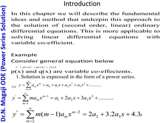
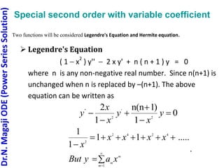
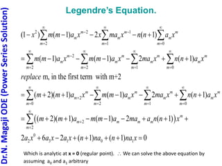
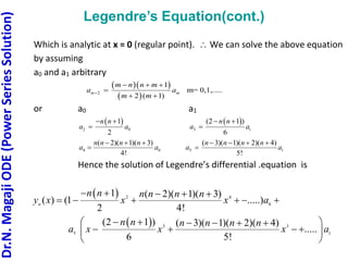
This document discusses power series solutions for second-order linear ordinary differential equations, focusing on variable coefficients and specific examples like Legendre's and Hermite's equations. It introduces methods to express solutions as power series and analyzes the derived Legendre polynomials and Hermite polynomials, emphasizing their applications in various mathematical and physical contexts. The solutions provided are derived through methods involving arbitrary constants and recurrence relations.

1. Dr.N.
Magaji
ODE
(Power
Series
Solution)
EGR 3301
Chapter 3
Power Series Solution of differential
equations

2. Dr.N.
Magaji
ODE
(Power
Series
Solution) Introduction
In this chapter we will describe the fundamental
ideas and method that underpin this approach to
the solution of (second order, linear) ordinary
differential equations. This is more applicable to
solving linear differential equations with
variable co-efficient.
Example
Consider general equation below
'' '
( ) ( ) ( )
y p x y q x y f x
  
p(x) and q(x) are variable co-effecients.
1. Solution is expressed in the form of a power series.
Let
2 3
0 1 2 3
0
..........
m
m
m
y a x a a x a x a x


     

' 1 2
1 2 3
1
2 3 ..........
m
m
m
y ma x a a x a x



    

'' 2 2
2 3 4
2
( 1) 2 3.2 4.3 ......
m
m
m
y m m a x a a x a x



    


3. Dr.N.
Magaji
ODE
(Power
Series
Solution)
Special second order with variable coefficient
Two functions will be considered Legendre's Equation and Hermite equation.
 Legendre's Equation
( 1  x
2
) y''  2 x y' + n ( n + 1 ) y = 0
where n is any non-negative real number. Since n(n+1) is
unchanged when n is replaced by –(n+1). The above
equation can be written as
'' '
2 2
2 n(n 1)
0
1 1
x
y y y
x x

  
 
4 2 4
1
2
2
1 1 .....
1
1
m
m
m
x x x x
But y a x
x


   
  

 .

4. Dr.N.
Magaji
ODE
(Power
Series
Solution)
Legendre’s Equation.
2 2 1
2 1 0
2
2 2 1 0
2
0 2
(1 ) ( 1) 2 ( 1)
( 1) ( 1) 2 ( 1)
m, in the first term with m+2
( 2)( 1) ( 1) 2
m m m
m m m
m m m
m m m m
m m m m
m m m m
m m m
m m m
m m m
x m m a x x ma x n n a x
m m a x m m a x ma x n n a x
replace
m m a x m m a x ma x
  
 
  
   

   
 

 
    
      
     
  
   
 
 
1 0
2
2
0
2 3 1 0 1
( 1)
( 2)( 1) ( 1) 2 ( 1)
2 6 2 ( 1) ( 1) 0
m
m
m
m
m m m m
m
n n a x
m m a m m a ma a n n x
a x a x a x n na n na x
 
 



 
        
      
 

Which is analytic at x = 0 (regular point). We can solve the above equation by
assuming a0 and a1 arbitrary

5. Dr.N.
Magaji
ODE
(Power
Series
Solution)
Legendre’s Equation(cont.)
Which is analytic at x = 0 (regular point). We can solve the above equation
by assuming
a0 and a1 arbitrary
  
 
2 m= 0,
1
2 ( 1)
1,.....
m m
m n n m
a a
m m

  

 
or a0 a1
 
2 0
1
2
n n
a a
 

 
3 1
(2 1 )
6
n n
a a
 

4 0
( 2)( 1)( 3)
4!
n n n n
a a
  
 5 1
( 3)( 1)( 2)( 4)
5!
n n n n
a a
   

Hence the solution of Legendre’s differential .equation is
 
 
0
1
4
3 3
5
2 ( 2)( 1)( 3)
.....)
4!
( 3)( 1)( 2)( 4)
1
( ) (1
2
(2 1 )
.....
5!
6
n
n n n n
a
n n
y x x x
n n
a x x x
n
a
n n n
  
   

 
 
 
 
   





 

6. Dr.N.
Magaji
ODE
(Power
Series
Solution)
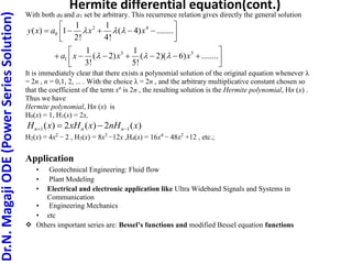
Legendre’s Equation(cont.)
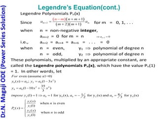
The general solution is y = a0 y1 + a1 y2
where
2 4 6
1
( 1) ( 2)( 1)( 3) ( -2)( -4)( 1)( 3)( 5)
( ) 1
2! 4! 6!
n n n n n n n n n n n n
y x x x x
      
    
3 5
2
7
( 1)( 2) ( 1)( 3)( 2)( 4)
( )
3! 5!
( 1)( 3)( 5)( 2)( 4)( 6)
7!
n n n n n n
y x x x x
n n n n n n
x
     
  
     
 
If n = 0, 1, 2, . . . (non-negative integer), then
y = c1 Pn(x) + c2 Qn(x)
where Pn(x) = Legendre polynomials [It is desirable that Pn(1) = 1]
Qn(x) = Legendre functions of the second kind converges in -
1<x<1, but Qn(1) = unbounded (This is due to the fact
that the Legendre equation is not analytic at x=+1 and
x=-1!)

7. Dr.N.
Magaji
ODE
(Power
Series
Solution)
Legendre’s Equation(cont.)
Legendre Polynomials Pn(x)
Since
  
  
2
1
2 1
m m
n m
a a
m m
n m

 

 

for m = 0, 1, . . .
when n = non-negative integer,
am+2 = 0 for m = n 2 0
n
a 
 
i.e., an+2 = an+4 = an+6 = . . . = 0
when n = even, y1  polynomial of degree n
n = odd, y2  polynomial of degree n
These polynomials, multiplied by an appropriate constant, are
called the Legendre polynomials Pn(x), which have the value Pn(1)
= 1. In other words, let
2
0 0 2 0
2 4
4 0
0 0 0 2 0 4
1
1
2
2
even (assume a1=0)
( ) ; (1 3 )
35
(1 10 )
3
8
1
(1) 1 1 for y (x), for y (x) and for y (x)
2 3
( )
when is even
(1)
( )
( )
when is odd
(1)
n
n
For
y x a y a x
y a x x
impose y a a a
y x
n
y
P x
y x
n
y
  
  
     



 




8. Dr.N.
Magaji
ODE
(Power
Series
Solution)
Legendre’s Equation(cont.)
   
   
2 4 2
0 2 4
1 3 5 0
3 5 3
1 1 3 1 5 1
1
1 1
( ) 1; ( ) (3 1); 35 30 3
2 8
polynomials of even degree
To get y (x),y (x) and y (x) assume a =0
5 21 14
( ) a ; y ( ) a ( ); y a
3 5 3
(1) 1 to get which im
n
P x P x x P x x x
Legender
y x x x x x x x x x
impose y a
     
     

   
3 5 3
1 3 5
plies
1 1
( ) ; ( ) (5 3 ); 63 70 15
2 8
polynomials of odd degree
P x x P x x x P x x x x
Legender
     
The Legendre polynomials satisfy the following
   
2
1
1
2 !
n
n
n n n
d
P x x
n dx
 
 
 
 
Pn(x) = 
m=0
M
(  1 )
m ( 2 n  2 m ) !
2
n
m ! ( n  m ) ! ( n  2 m ) !
x
n-2m
where M =
when is even
2
1
when is odd
2
n
n
n
n









9. Dr.N.
Magaji
ODE
(Power
Series
Solution)
Legendre’s Equation(cont.)
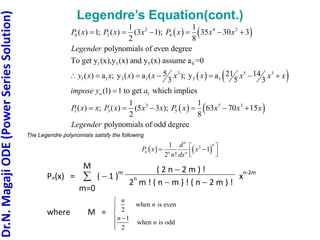
Then, the Legendre polynomial of degree n, Pn(x) is given by
[Example]
   
   
2
0 1 2
3 4 2
3 4
5 3
5
1
( ) 1; ( ) ; ( ) (3 1)
2
1 1
( ) (5 3 ); 35 30 3
2 8
1
63 70 15
8
P x P x x P x x
P x x x P x x x
P x x x x
   
    
  
Application
 Steady state temperatures within a solid spherical ball when the
temperature at points of its boundary is known.
 Solving Laplace’s equation in spherical coordinates.
 Quantum mechanical model of the hydrogen atom

10. Dr.N.
Magaji
ODE
(Power
Series
Solution) Hermite differential equation
Another standard second order ODE is
''
2 0 , ,
y xy y x


   
 

Which appears, most typically, in elementary solutions of Schrödinger’s equation;
λ is a parameter. This is Hermite’s equation, where special choices of λ give rise to
the Hermite polynomials. [Charles Hermite (1822-1901), French mathematician
who made important contributions to the theory of differential equations and also
worked on the theory of matrices.
Solution
2 3
0 1 2 3
0
..........
n
n
n
y a x a a x a x a x


     

which gives
2 1
2 1 0
2 0 2
1 1
( 1) 2 0
This is written as
2 ( 2)(m 1) (2 ) 0
m m m
m m m
m m m
m m
m m
m m
a m m x a mx a x
a a a m x a m x

 
  
 
  
 

 
   
       
  
 
Which is an identity for all values of x if am+2 (m+2)(m+1) =
am(2m−λ ) , m = 0,1,2, ... ,
2 2 0
n 1 0 2 1
(2 )
and
( 2)( 1) 2
y (x)=y a +y a
m m
m
a a a a
m m
 

 
 
 

11. Dr.N.
Magaji
ODE
(Power
Series
Solution) Hermite differential equation(cont.)
With both a0 and a1 set be arbitrary. This recurrence relation gives directly the general solution
2 4
0
3 5
1
1 1
( ) 1 ( 4) ........
2! 4!
1 1
( 2) ( 2)( 6) ........
3! 5!
y x a x x
a x x x
  
  
 
    
 
 
 
      
 
 
It is immediately clear that there exists a polynomial solution of the original equation whenever λ
= 2n , n = 0,1, 2, ... . With the choice λ = 2n , and the arbitrary multiplicative constant chosen so
that the coefficient of the term xn
is 2n , the resulting solution is the Hermite polynomial, Hn (x) .
Thus we have
Hermite polynomial, Hn (x) is
H0(x) = 1, H1(x) = 2x,
1 1
( ) 2 ( ) 2 ( )
n n n
H x xH x nH x
 
 
H2(x) = 4x2
− 2 , H3(x) = 8x3
−12x ,H4(x) = 16x4
− 48x2
+12 , etc.;
Application
• Geotechnical Engineering: Fluid flow
• Plant Modeling
• Electrical and electronic application like Ultra Wideband Signals and Systems in
Communication
• Engineering Mechanics
• etc
 Others important series are: Bessel’s functions and modified Bessel equation functions

12. Dr.N.
Magaji
ODE
(Power
Series
Solution) Hermite differential equation(cont.)
Exercises 1
1 Write down H5(x) .
2. Confirm that    
2 2
( ) 1 for n=0,1,2,3,4
n
n x x
n n
d
H x e e
dx

  (This is Rodrigues’ formula for the
Hermite polynomials.)
3 Show that fundamental system of solutions of Legendre Equation
2
(1 ) 2 ( 1) 0
x y xy p p y
 
     consists of
2
1
1
(1) ( 2 1)( 2 3) ( 1) ( 2) ( 2 2)
( ) 1
2 !
n
n
n
p n p n p p p p n
y x x
n


       
  
2 1
2
1
(1) ( 2 )( 2 2) ( 2)( 1) ( 2 1)
( )
(2 1)!
n
n
n
p n p n p p p n
y x x x
n



      
 

 .
3 Obtain the general solution of Hermite differential equation by power series method
5 Hermite’s equation is
2 2 0,
y xy py
 
  
where p is a constant.
a. Show that its general solution is 0 1 1 2
( ) ( ) ( )
y x a y x a y x
  , where
2 3
1
2 2 ( 2) 2 ( 2)( 4)
( ) 1 ...
2! 4! 6!
p p p p p p
y x
  
    
and
2 3
3 5 7
2
2( 1) 2 ( 1)( 3) 2 ( 1)( 3)( 5)
( ) ....
3! 5! 7!
p p p p p p
y x x x x x
     
    
converge for all x .