Downloaded 118 times
![2.3. LINEAR FIRST ORDER EQUATIONS
2.3
13
Linear First Order Equations
2.4
If a first order differential equation can be written in the form
y + p(x)y = r(x)
CHAPTER 2. EXACT EQUATIONS
Bernoulli Equation
The equation
y + p(x)y = g(x)y a
(2.7)
it is called a linear differential equation. If r(x) = 0, the equation is homogeneous, otherwise it is nonhomogeneous.
We can express the equation (2.7) as [p(x)y − r(x)]dx + dy = 0. This is
not exact but it has an integrating factor:
R = p(x), F = e
14
p dx
is called Bernoulli equation. It is nonlinear. Nonlinear equations are usually
much more difficult than linear ones, but Bernoulli equation is an exception.
It can be linearized by the substitution
u(x) = [y(x)]1−a
(2.14)
(2.8)
Then, we can solve it as other linear equations.
Method of Solution:
• Given a first order linear equation, express it in the following form:
y + p(x)y = r(x)
p dx
y +e
p dx
py = re
2
p dx
y −
ex
2x
y=
3
3xy 2
p(x) dx to
obtain
e
Example 2.5 Solve the equation
(2.9)
• Multiply both sides by the integrating factor F (x) = exp
(2.10)
Here a = −2 therefore u = y 1−(−2) = y 3 ⇒ u = 3y 2 y
Multiplying both sides of the equation by 3y 2 we obtain
2
• Express the left hand side as a single parenthesis.
e
p dx
y
= re
p dx
3y 2 y − 2xy 3 =
(2.11)
y(x) = e−h
eh r dx + c
(2.12)
2
ex
x
⇒
u − 2xu =
e
−2x dx
= e−x
2
2
Multiplying both sides by e−x , we get
2
p dx.
2
e−x u − 2xe−x u =
Example 2.4 Solve y + 4y = 1
2
The integrating factor is F = e
equation by e4x to obtain
4 dx
(e−x u) =
4x
= e . Multiply both sides of the
2
e4x y + 4e4x y =e4x
e−x u = ln x + c
⇒
⇒
1
y = + ce−4x
4
1
x
1
x
u = (ln x + c)ex
(e4x y) =e4x
e4x
e4x y =
+c
4
ex
x
This equation is linear. Its integrating factor is
• Integrate both sides. Don’t forget the integration constant. The solution is:
where h =
(2.13)
y = (ln x + c)ex
2
1/3
2](https://image.slidesharecdn.com/258lecnot2-131215083806-phpapp02/75/258-lecnot2-12-2048.jpg)
![EXERCISES
15
16
Exercises
Answers
Solve the following differential equations. (Find an integrating factor if
necessary)
1) (yex + xyex + 1)dx + xex dy = 0
2) (2r + 2 cos θ)dr − 2r sin θdθ = 0
3) (sin xy + xy cos xy)dx + (x2 cos xy)dy = 0
4) 2 cos ydx = sin ydy
5) 5dx − ey−x dy = 0
6) (2xy + 3x2 y 6 ) dx + (4x2 + 9x3 y 5 ) dy = 0
7) (3xey + 2y) dx + (x2 ey + x) dy = 0
1
5
8) y + y =
x
x
9) y +
1
1
y=
x ln x
ln x
c
− 1 e−x
x
r2 + 2r cos θ = c
x sin xy = c
F = e2x , e2x cos y = c
F = ex , 5ex − ey = c
F = y 3 , x 2 y 4 + x3 y 9 = c
F = x, x3 ey + x2 y = c
c
1
y= + 5
5 x
1) y =
2)
3)
4)
5)
6)
7)
8)
9) y =
x+c
ln x
10) y = −1 +
x4
12) y = 4 − 5e− 4
Reduce to linear form and solve the following equations:
2 sin x 1/2
13) y − 4y tan x =
y
cos3 x
x
y
5 ln x 4/5
25
y=
y
15) y +
x
x5
13) y =
14) y =
c − ln cos x
cos2 x
1
2
2
− x + ce−2x
15) y =
y
1
=− 9 3
x
xy
x ln x − x + c
x5
16) y =
14) y + y = −
1
c
+ 4
8
x
x
19) x = y −2
2
1/4
1
3
cosh 3y + c
Hint: x ↔ y
20) y =
20) 2xyy + (x − 1)y 2 = x2 ex
5
17) y = arcsin[c(x − 1)]
1
c
+ 3
18) F = y, x =
2y y
tan y
17) y =
x−1
18) y 2 dx + (3xy − 1)dy = 0
19) y (sinh 3y − 2xy) = y
c
cos x
11) y = x4 cos x + c cos x
10) y − y tan x = tan x
11) y + y tan x = 4x3 cos x
12) y + x3 y = 4x3 , y(0) = −1
16) y +
CHAPTER 2. EXACT EQUATIONS
Hint: z = y 2
cxe−x + 1 xex
2](https://image.slidesharecdn.com/258lecnot2-131215083806-phpapp02/75/258-lecnot2-13-2048.jpg)
![3.3. CONSTANT COEFFICIENTS
21
Double Real Root: One solution is eλx but we know that a second order
equation must have two independent solutions. Let’s use the method of
reduction of order to find the second solution.
y − 2ay + a2 y = 0
⇒
y1 = eax
(3.10)
22
CHAPTER 3. SECOND ORDER EQUATIONS
3.4
Cauchy-Euler Equation
The equation x2 y + axy + by = 0 is called the Cauchy-Euler equation. By
inspection, we can easily see that the solution must be a power of x. Let’s
substitute y = xr in the equation and try to determine r. We will obtain
Let’s insert y2 = ueax in the equation.
r(r − 1)xr + arxr + bxr = 0
ax
ax
e u + (2a − 2a)e u = 0
Obviously, u = 0 therefore u = c1 + c2 x. The general solution is
y = c1 eλx + c2 xeλx
(3.12)
Example 3.4 Solve y + 2y + y = 0
λx
r2 + (a − 1)r + b = 0
(3.11)
(3.17)
(3.18)
This is called the auxiliary equation. Once again, we have three different
cases according to the types of roots. The general solution is given as follows:
• Two real roots
2
y = e . The characteristic equation is λ + 2λ + 1 = 0. Its solution is the
double root λ = −1, therefore the general solution is
y = c1 e−x + c2 xe−x
(3.13)
This can be proved using Taylor series expansions.
If the solution of the characteristic equation is
λ1 = α + iβ, λ2 = α − iβ
y = c1 e
(cos βx + i sin βx) + c2 e
αx
(cos βx − i sin βx)
(3.14)
(3.15)
By choosing new constants A, B, we can express this as
y=e
αx
(A cos βx + B sin βx)
y = c1 xr + c2 xr ln x
(3.20)
• Complex conjugate roots where r1 , r2 = r ± si
y = xr [c1 cos(s ln x) + c2 sin(s ln x)]
then the general solution of the differential equation will be
αx
(3.19)
• Double real root
Complex Conjugate Roots: We need the complex exponentials for this
case. Euler’s formula is
eix = cos x + i sin x
y = c1 xr1 + c2 xr2
(3.21)
Example 3.6 Solve x2 y + 2xy − 6y = 0
Insert y = xr . Auxiliary equation is r2 + r − 6 = 0. The roots are
r = 2, r = −3 therefore
y = c1 x2 + c2 x−3
(3.16)
Example 3.5 Solve y − 4y + 29y = 0.
Example 3.7 Solve x2 y − 9xy + 25y = 0
y = eλx . The characteristic equation is λ2 −4λ+29 = 0. Therefore λ = 2±5i.
The general solution is
Insert y = xr . Auxiliary equation is r2 − 10r + 25 = 0. Auxiliary equation
has the double root r = 5 therefore the general solution is
y = e2x (A cos 5x + B sin 5x)
y = c1 x5 + c2 x5 ln x](https://image.slidesharecdn.com/258lecnot2-131215083806-phpapp02/75/258-lecnot2-16-2048.jpg)
![EXERCISES
23
24
Exercises
CHAPTER 3. SECOND ORDER EQUATIONS
Answers
1)
2)
3)
4)
5)
Are the following sets linearly independent?
1) {x4 , x8 }
2) {sin x, sin2 x}
3) {ln(x5 ), ln x}
Use reduction of order to find a second linearly independent solution:
4) x2 (ln x − 1) y − xy + y = 0,
y1 = x
1
5) x2 ln x y + (2x ln x − x)y − y = 0,
y1 =
x
6) y + 3 tan x y + (3 tan2 x + 1)y = 0,
y1 = cos x
Yes
Yes
No
y2 = ln x
y2 = ln x − 1
6) y2 = sin x cos x
7) y = (1 + x)e−x
1
8) y = c1 e−2x + c2 e− 2 x
Solve the following equations:
7) y + 2y + y = 0, y(0) = 1, y (0) = 0
9) y = e8x
5
8) y + y + y = 0
2
10) y = c1 e−12x + c2 xe−12x
9) y − 64y = 0, y(0) = 1,
10) y + 24y + 144y = 0
y (0) = 8
11) y = 4e−x + 3xe−x
7
11) y + 2y + y = 0, y(−1) = e, y(1) =
e
12) 5y − 8y + 5y = 0
π2
13) y + 2y + 1 +
y = 0, y(0) = 1, y (0) = −1
4
14) y − 2y + 2y = 0, y(π) = 0, y(−π) = 0
15) xy + y = 0
16) x2 y − 3xy + 5y = 0
17) x2 y − 10xy + 18y = 0
18) x2 y − 13xy + 49y = 0
19) Show that y1 = u and y2 = u
y −
v
u
+2
v
u
y +
12) y = e0.8x [A cos(0.6x) + B sin(0.6x)]
13) y = e−x cos
14) y = ex sin x
15) y = c1 + c2 ln x
16) y = x2 [c1 cos(ln x) + c2 sin(ln x)]
vdx are solutions of the equation
vu
u2 u
+2 2 −
vu
u
u
π
x
2
y=0
20) Show that y1 = u and y2 = v are solutions of the equation
(uv − vu )y + (vu − uv )y + (u v − v u )y = 0
17) y = c1 x2 + c2 x9
18) y = c1 x7 + c2 x7 ln x](https://image.slidesharecdn.com/258lecnot2-131215083806-phpapp02/75/258-lecnot2-17-2048.jpg)
![EXERCISES
39
Exercises
CHAPTER 5. HIGHER ORDER EQUATIONS
Answers
1) y = c0 + c1 x + c2 x2 + c3 x3 + c4 x4
1) D5 y = 0
2) y = c1 ex + c2 xex + c3 x2 ex
2) (D − 1)3 y = 0
3) y − 4y + 13y = 0
4) (D − 2)2 (D + 3)3 y = 0
5) (D2 + 2)3 y = 0
d4 y
d2 y
+ 5 2 + 4y = 0
dx4
dx
7) (D2 + 9)2 (D2 − 9)2 y = 0
6)
4
40
3
2
dy
dy
dy
−2 3 +2 2 =0
4
dx
dx
dx
9) y − 3y + 12y − 10y = 0
8)
3) y = c1 e2x cos 3x + c2 e2x sin 3x + c3
4) y = c1 e2x + c2 xe2x + c3 e−3x + c4 xe−3x + c5 x2 e−3x
√
√
√
√
5) y = c1 cos 2x + c2 sin 2x + c3 x cos 2x + c4 x sin 2x
√
√
+ c5 x2 cos 2x + c6 x2 sin 2x
6) y = c1 cos 2x + c2 sin 2x + c3 cos x + c4 sin x
7) y = c1 e3x + c2 xe3x + c3 e−3x + c4 xe−3x + c5 cos 3x + c6 sin 3x
+ c7 x cos 3x + c8 x sin 3x
8) y = c1 + c2 x + c3 ex cos x + c4 ex sin x
10) (D2 + 2D + 17)2 y = 0
9) y = c1 ex + c2 ex cos 3x + c3 ex sin 3x
11) (D4 + 2D2 + 1)y = x2
10) y = c1 e−x sin 4x + c2 e−x cos 4x + c3 xe−x sin 4x + c4 xe−x cos 4x
12) (D3 + 2D2 − D − 2)y = 1 − 4x3
11) y = c1 cos x + c2 sin x + c3 x cos x + c4 x sin x + x2 − 4
√
√
√
13) (2D4 + 4D3 + 8D2 )y = 40e−x [ 3 sin( 3x) + 3 cos( 3x)]
14) (D3 − 4D2 + 5D − 2)y = 4 cos x + sin x
15) (D3 − 9D)y = 8xex
12) y = c1 ex + c2 e−x + c3 e−2x + 2x3 − 3x2 + 15x − 8
√
√
√
13) y = c1 + c2 x + c3 e−x cos 3x + c4 e−x sin 3x + 5xe−x cos 3x
14) y = c1 ex + c2 xex + c3 e2x + 0.2 cos x + 0.9 sin x
3
15) y = c1 + c2 e3x + c3 e−3x + ex − xex
4](https://image.slidesharecdn.com/258lecnot2-131215083806-phpapp02/75/258-lecnot2-25-2048.jpg)
![6.2. CLASSIFICATION OF POINTS
6.2
43
Classification of Points
44
CHAPTER 6. SERIES SOLUTIONS
Example 6.1 Solve y + 2xy + 2y = 0 around x0 = 0.
First we should classify the point. Obviously, x = 0 is an ordinary point, so
we can use power series method.
Consider the equation
R(x)y + P (x)y + Q(x)y = 0
(6.2)
∞
∞
n
y=
If both of the functions
P (x)
,
R(x)
Q(x)
R(x)
an x , y =
n=0
(6.3)
are analytic at x = x0 , then the point x0 is an ordinary point. Otherwise, x0
is a singular point.
Suppose that x0 is a singular point of the above equation. If both of the
functions
Q(x)
P (x)
, (x − x0 )2
(6.4)
(x − x0 )
R(x)
R(x)
are analytic at x = x0 , then the point x0 is called a regular singular point.
Otherwise, x0 is an irregular singular point.
For example, the functions 1+x+x2 , sin x, ex (1+x4 ) cos x are all analytic
cos x 1 ex 1 + x2
at x = 0. But, the functions
, ,
,
are not.
x
x x
x3
We will use power series method around ordinary points and Frobenius’
method around regular singular points. We will not consider irregular singular points.
∞
nan x
n−1
n(n − 1)an xn−2
, y =
n=1
n=2
Inserting these in the equation, we obtain
∞
∞
n(n − 1)an x
n−2
∞
+ 2x
n=2
nan x
n−1
an x n = 0
+2
n=1
∞
n=0
∞
∞
n(n − 1)an xn−2 +
n=2
2nan xn +
n=1
2an xn = 0
n=0
To equate the powers of x, let us replace n by n + 2 in the first sigma.
(n → n + 2)
∞
∞
∞
n=1
n=0
2an xn = 0
2nan xn +
(n + 2)(n + 1)an+2 xn +
n=0
Now we can express the equation using a single sigma, but we should start
the index from n = 1. Therefore we have to write n = 0 terms separately.
∞
[(n + 2)(n + 1)an+2 + (2n + 2)an ] xn = 0
2a2 + 2a0 +
n=1
6.3
Power Series Method
If x0 is an ordinary point of the equation R(x)y + P (x)y + Q(x)y = 0, then
the general solution is
∞
an (x − x0 )n
y=
−2(n + 1)
−2
an =
an
(n + 2)(n + 1)
(n + 2)
This is called the recursion relation. Using it, we can find all the constants
in terms of a0 and a1 .
a2 = −a0 , an+2 =
(6.5)
2
1
a4 = − a2 = a0
4
2
2
1
a6 = − a4 = − a0
6
6
2
a3 = − a1 ,
3
2
4
a 5 = − a3 = a1
5
15
n=0
The coefficients an can be found by inserting y in the equation and setting
the coefficients of all powers to zero. Two coefficients (Usually a0 and a1 )
must be arbitrary, others must be defined in terms of them. We expect two
linearly independent solutions because the equation is second order linear.
We can find as many coefficients as we want in this way. Collecting them
together, the solution is :
1
1
y = a0 1 − x 2 + x 4 − x 6 + · · ·
2
6
2
4
+ a1 x − x 3 + x 5 + · · ·
3
15](https://image.slidesharecdn.com/258lecnot2-131215083806-phpapp02/75/258-lecnot2-27-2048.jpg)
![6.3. POWER SERIES METHOD
45
In most applications, we want a solution close to 0, therefore we can neglect
the higher order terms of the series.
Remark: Sometimes we can express the solution in closed form (in terms
of elementary functions rather than an infinite summation) as in the next
example:
Example 6.2 Solve (x − 1)y + 2y = 0 around x0 = 0.
Once again, first we should classify the given point. The function
analytic at x = 0, therefore x = 0 is an ordinary point.
∞
∞
∞
an x n , y =
y=
n=0
2
is
x−1
nan xn−1 , y =
n=1
n(n − 1)an xn−2
n=2
Inserting these in the equation, we obtain
∞
(x − 1)
∞
n(n − 1)an x
n−2
nan xn−1 = 0
+2
n=2
n=1
∞
∞
∞
n(n − 1)an xn−2 +
n(n − 1)an xn−1 −
n=1
n=2
n=2
2nan xn−1 = 0
46
CHAPTER 6. SERIES SOLUTIONS
Exercises
Find the general solution of the following differential equations in the
form of series. Find solutions around the origin (use x0 = 0). Write the
solution in closed form if possible.
1) (1 − x2 )y − 2xy = 0
2) y + x4 y + 4x3 y = 0
3) (2 + x3 )y + 6x2 y + 6xy = 0
4) (1 + x2 )y − xy − 3y = 0
5) (1 + 2x2 )y + xy + 2y = 0
6) y − xy + ky = 0
7) (1 + x2 )y − 4xy + 6y = 0
8) (1 − 2x2 )y + (2x + 4x3 )y − (2 + 4x2 )y = 0
9) (1 + 8x2 )y − 16y = 0
10) y + x2 y = 0
The following equations give certain special functions that are very important in applications. Solve them for n = 1, 2, 3 around origin. Find
polynomial solutions only.
To equate the powers of x, let us replace n by n+1 in the second summation.
∞
∞
n(n − 1)an x
n−1
−
n=2
∞
(n + 1)nan+1 x
n−1
+
n=1
2nan x
n−1
=0
n=1
Now we can express the equation using a single sigma.
11)
12)
13)
14)
(1 − x2 )y − 2xy + n(n + 1)y = 0
y − 2xy + 2ny = 0
xy + (1 − x)y + ny = 0
(1 − x2 )y − xy + n2 y = 0
(Legendre’s Equation)
(Hermite’s Equation)
(Laguerre’s Equation)
(Chebyshev’s Equation)
∞
[(n(n − 1) + 2n)an − n(n + 1)an+1 ] xn−1 = 0
(−2a2 + 2a1 ) +
n=2
a2 = a1 , an+1 =
n2 − n + 2n
an for n
n(n + 1)
2
So the recursion relation is:
an+1 = an
All the coefficients are equal to a1 , except a0 . We have no information about
it, so it must be arbitrary. Therefore, the solution is:
y = a0 + a1 x + x 2 + x 3 + · · ·
x
y = a0 + a1
1−x
Solve the following initial value problems. Find the solution around the
point where initial conditions are given.
15)
16)
17)
18)
xy + (x + 1)y − 2y = 0,
y + 2xy − 4y = 0,
4y + 3xy − 6y = 0,
(x2 − 4x + 7)y + y = 0,
x0
x0
x0
x0
= −1,
= 0,
=0
=2
y(−1) = 1,
y(0) = 1,
y(0) = 4,
y(2) = 4,
y (−1) = 0
y (0) = 0
y (0) = 0
y (2) = 10
19) Find the recursion relation for (p + x2 )y + (1 − q − r)xy + qry = 0
around x = 0. (Here p, q, r are real numbers, p = 0)
20) Solve (1 + ax2 )y + bxy + cy = 0 around x0 = 0](https://image.slidesharecdn.com/258lecnot2-131215083806-phpapp02/75/258-lecnot2-28-2048.jpg)


![7.2. EXAMPLES
51
∞
∞
4(n + r)(n + r − 1)an x
n+r−1
∞
+
n=0
2(n + r)an x
n=0
n+r−1
an xn+r = 0
+
52
CHAPTER 7. FROBENIUS’ METHOD
For simplicity, we may choose a0 = 1. Then
an =
We want to equate the powers of x, so n → n + 1 in the first two terms.
∞
∞
∞
4(n + r + 1)(n + r)an+1 xn+r +
n=−1
2(n + r + 1)an+1 xn+r +
n=−1
an xn+r = 0
Therefore the second solution is :
∞
n=0
Now we can express the equation using a single sigma, but the index of the
common sigma must start from n = 0. Therefore we have to write n = −1
terms separately.
[4r(r−1)+2r]a0 xr−1 +
{[4(n + r + 1)(n + r) + 2(n + r + 1)]an+1 + an } xn+r = 0
n=0
We know that a0 = 0, therefore 4r2 − 2r = 0. This is the indicial equation.
Its solutions are r = 0, r = 1 . Therefore this is Case 1.
2
If r = 0, the recursion relation is
n=0
The general solution is y = c1 y1 + c2 y2
2
First we should classify the given point. The function x x−x is not analytic
2
at x = 0 therefore x = 0 is a singular point. The functions x − 1 and
1 + x are analytic at x = 0 therefore x = 0 is a R.S.P., we can use the
method of Frobenius. Evaluating the derivatives of y and inserting them in
the equation, we obtain
−1
1 an
4(n + 1)(n + 2 )
an+1 =
∞
For simplicity, we may choose a0 = 1. Then
n=0
∞
−
(n + r)an x
(−1)
2n!
y1 =
n=0
n=0
+
an x
n+r
∞
an xn+r+1 = 0
+
n=0
n=0
∞
∞
(n + r)(n + r − 1)an x
n=0
∞
n n
(n + r)an xn+r+1
+
Let’s replace n by n − 1 in the second and fifth terms.
Therefore the first solution is:
∞
n+r
∞
n+r
n=0
n
an =
∞
(n + r)(n + r − 1)an x
a0
a1
a0
a2
a0
a1 = − , a 2 = −
, a3 = −
,...
3 =
5 = −
2
4!
6!
4.2. 2
4.3. 2
−
√
(−1) x
= cos x
2n!
1
If r = , the recursion relation is
2
a1 = −
√
(−1)n xn
= sin x
(2n + 1)!
y2 = x1/2
Example 7.2 Solve x2 y + (x2 − x)y + (1 + x)y = 0 around x0 = 0.
∞
an+1 =
(−1)n
(2n + 1)!
n=0
−1
−an
an =
(2n + 3)(2n + 2)
4(n + 3 )(n + 1)
2
a0
a1
a0
a2
a0
, a2 = −
= , a3 = −
= − ,...
3.2
5.4
5!
7.6
7!
n+r
n=1
∞
(n + r)an x
n=0
n+r
an x
+
n=0
(n + r − 1)an−1 xn+r
+
n+r
∞
an−1 xn+r = 0
+
n=1
[r2 − 2r + 1]a0 xr +
∞
{[(n + r)(n + r − 1) − (n + r) + 1]an + [(n + r − 1) + 1]an−1 } xn+r = 0
n=1
The indicial equation is r2 − 2r + 1 = 0 ⇒ r = 1 (double root). Therefore
this is Case 2. The recursion relation is
an = −
n+1
an−1
n2](https://image.slidesharecdn.com/258lecnot2-131215083806-phpapp02/75/258-lecnot2-31-2048.jpg)
![7.2. EXAMPLES
53
54
CHAPTER 7. FROBENIUS’ METHOD
Exercises
For simplicity, let a0 = 1. Then
3
3
4
2
a1 = −2, a2 = − a1 = , a3 = − a2 = −
4
2
9
3
Find two linearly independent solutions of the following differential equations in the form of series. Find solutions around the origin (use x0 = 0).
Write the solution in closed form if possible.
1) 2x2 y − xy + (1 + x)y = 0
Therefore the first solution is :
3
2
y1 = x 1 − 2x + x2 − x3 + · · ·
2
3
2) 2xy + (1 + x)y − 2y = 0
To find the second solution, we will use reduction of order. Let y2 = uy1 .
Inserting y2 in the equation, we obtain
3) (x2 + 2x)y + (3x + 1)y + y = 0
4) xy − y − 4x3 y = 0
2
2
2
x y1 u + (2x y1 − xy1 + x y1 )u = 0
Let w = u then
−2
To evaluate the integral u =
1−x+
w=
u=
1
x
⇒
w=
8) (2x2 + 2x)y − y − 4y = 0
xe−x
2
y1
9) 2x2 y + (2x2 − x)y + y = 0
1
w dx we need to find 2 . This is also a series.
y1
3
2
1 − 2x + x2 − x3 + · · ·
2
3
xe−x
=x
2
y1
7) x2 y + (x2 − x)y + y = 0
y1 1
+ − 1 dx
y1 x
ln w = −2 ln y1 + ln x − x
w=
6) 3x2 y + (−10x − 3x2 )y + (14 + 4x)y = 0
1
y
w + 2 1 − +1 w =0
y1 x
dw
=
w
1
1
= 2
2
y1
x
5) xy + y − xy = 0
−2
=
x2 x3
−
+ ···
2!
3!
1 + 3x +
1
x2
1
x2
1 + 4x + 9x2 +
1 + 4x + 9x2 +
11 2 13 3
x + x + ···
2
6
w dx = ln x + 3x +
11 2 13 3
x + x + ···
4
18
13
3
y2 = uy1 = y1 ln x + x 3x − x2 + x3 + · · ·
4
2
46 3
x + ···
3
46 3
x + ···
3
10) 4x2 y + (2x2 − 10x)y + (12 − x)y = 0
11) (x2 + 2x)y + (4x + 1)y + 2y = 0
Use Frobenius’ method to solve the following differential equations around
origin. Find the roots of the indicial equation, find the recursion relation,
and two linearly independent solutions.
12) (x2 + cx)y + [(2 + b)x + c(1 − d)]y + by = 0
(b = 0, c = 0, d is not an integer).
13) x2 y + [(1 − b − d)x + cx2 ]y + [bd + (1 − b)cx]y = 0
(c = 0, b − d is not an integer).
14) x2 y + [(1 − 2d)x + cx2 ]y + (d2 + (1 − d)cx)y = 0
(c = 0)
15) xy + [1 − d + cx2 ]y + 2cxy = 0
(c = 0, d is not an integer).](https://image.slidesharecdn.com/258lecnot2-131215083806-phpapp02/75/258-lecnot2-32-2048.jpg)
![58
CHAPTER 8. LAPLACE TRANSFORM I
Example 8.1 Evaluate the Laplace transform of the following functions:
a) f (t) = 1
∞
0
Chapter 8
0
1
= ,
s
s>0
b) f (t) = eat
∞
Laplace Transform I
0
c) f (t) =
Laplace transform provides an alternative method for many equations. We
first transform the differential equation to an algebraic equation, then solve
it, and then make an inverse transform. Laplace transform has a lot of
interesting properties that make these operations easy. In this chapter, we
will see the definition and the basic properties. We will also compare this
method to the method of undetermined coefficients, and see in what ways
Laplace transform is more convenient.
0
1
if
if
∞
1
∞
e−st f (t)dt
(8.1)
0
then, the inverse transform will be
f (t) = L−1 {F (s)}
(8.2)
Note that we use lowercase letters for functions and capital letters for their
transforms.
57
=
0
1
, s>a
s−a
∞
=
1
e−s
,
s
s>0
d) f (t) = t
∞
te−st dt
L {t} =
0
Using integration by parts, we obtain
L {t} = −
The Laplace transform of a function f (t) is defined as:
e−st
−s
e−st dt =
L {f } =
Definition, Existence and Inverse of Laplace
Transform
∞
0<t<1
1 t
L {t} = −t
F (s) = L {f (t)} =
e(a−s)t
a−s
eat e−st dt =
L eat =
8.1
∞
e−st
−s
e−st dt =
L {1} =
e−st
s
∞
e−st
s2
∞
∞
+
0
0
=
0
e−st
dt
s
1
, s>0
s2
The integral that defines the Laplace transform is an improper integral,
it may or may not converge. In the above examples, the transform is defined
for a certain range of s.
In practice, we can use Laplace transform on most of the functions we
encounter in differential equations. The following definitions and the theorem
answer the question Which functions have a Laplace transform?
Piecewise Continuous Functions: A function f (t) is piecewise continuous
on [a, b] if the interval can be subdivided into subintervals [ti , tj ],
a = t0 < t1 < t2 · · · < tn = b such that f (t) is continuous on each interval
and has finite one-sided limits at the endpoints (from the interior).
An example can be seen on Figure 8.1.](https://image.slidesharecdn.com/258lecnot2-131215083806-phpapp02/75/258-lecnot2-34-2048.jpg)
![8.2. PROPERTIES
59
60
CHAPTER 8. LAPLACE TRANSFORM I
• Transform of Derivatives
L {f }
L {f }
L f (n)
= sL {f } − f (0)
= s2 L {f } − sf (0) − f (0)
= sn L {f } − sn−1 f (0) − sn−2 f (0) − · · · − f (n−1) (0)
• Transform of Integrals
t
L
f (x) dx
=
0
F (s)
s
Example 8.2 Find the Laplace transform of sin at and cos at. Hint: Use
Euler’s formula eix = cos x + i sin x and linearity.
Figure 8.1: A piecewise continuous function
Exponential Order: f (t) is of exponential order as t → ∞ if there exist
real constants M, c, T such that |f (t)| M ect for all t T . In other words,
a function is of exponential order if it does not grow faster than ect .
Theorem 8.1: If f (t) is of exponential order and piecewise continuous on
[0, k] for all k > 0, then its Laplace transform exists for all s > c.
For example, all the polynomials have a Laplace transform. The function
t2
e does NOT have a Laplace transform.
8.2
Basic Properties of Laplace Transforms
It is difficult to evaluate the Laplace transform of each function by performing an integration. Instead of this, we use various properties of Laplace
transform.
Let L {f (t)} = F (s), then, some basic properties are: (assuming these
transforms exists)
• Linearity
L {af + bg} = aL {f } + bL {g}
• Shifting
L {eiat } − L {e−iat }
2i
1
1
1
a
L {sin at} =
−
= 2
2i s − ia s + ia
s + a2
Similarly, we can show that the transform of f (t) = cos at is
s
F (s) = 2
s + a2
1
Example 8.3 Find the inverse Laplace transform of F (s) =
.
(s + 5)2
Hint: Use shifting.
sin at =
eiat − e−iat
2i
We know that L−1
1
s2
L−1 {F (s − a)} = eat f (t)
L {sin at} =
= t. Therefore
1
(s + 5)2
L−1
= te−5t
Example 8.4 Find the Laplace transform of f (t) = t2 . Hint: Use Derivatives.
Using L {f } = sL {f } − f (0), we obtain
L {2t}
2
= 3
s
s
Example 8.5 Find the Laplace transform of f (t) = t3 . Hint: Use Integrals.
L {2t} = sL t2 − 0
⇒
L t2 =
Using the integral rule, we see that
L
L eat f (t) = F (s − a)
⇒
L {t2 }
2
= 4
s
s
6
L t3 = 4
s
t3
3
=](https://image.slidesharecdn.com/258lecnot2-131215083806-phpapp02/75/258-lecnot2-35-2048.jpg)
![68
CHAPTER 9. LAPLACE TRANSFORM II
Reversing the order of integration, we obtain:
∞
∞
f (x) g(t − x)e−st dt dx
=
0
x
Making the substitution u = t − x, we obtain:
∞
∞
f (x) g(u)e−su−sx dudx
L {f ∗ g} =
Chapter 9
0
∞
0
∞
0
0
Laplace Transform II
g(u)e−su du
f (x)e−sx dx
=
=F (s) G(s)
Example 9.1 Find the inverse Laplace transform of F (s) =
In this chapter, we will study more advanced properties of Laplace transform.
At the end, we will be able to find transform and inverse transform of a wider
range of functions. This will enable us to solve almost any linear constant
coefficient equation, including discontinuous inputs.
9.1
L−1
1
s2
1
s+4
= t, L−1
t
(9.1)
0
The convolution operation is commutative, in other words f ∗ g = g ∗ f
Theorem 9.1: The transform of convolution of two functions is equal to
the product of their transforms, i.e.
L {f ∗ g} = F (s) · G(s)
−1
L
{F (s) · G(s)} = f ∗ g
where L {f } = F (s) and L {g} = G(s).
Proof: Using the definitions of convolution and Laplace transform,
t
L {f ∗ g} =L
f (x) g(t − x) dx
0
∞
t
f (x) g(t − x)e−st dx dt
=
0
0
67
L−1
1
1
·
2 s+4
s
(9.2)
(9.3)
= t ∗ e−4t
xe−4(t−x) dx
0
xe4x e4x
−
4
16
−4t
t
1
e
= −
+
4 16
16
t
= e−4t
0
Example 9.2 Find the inverse Laplace transform of F (s) =
The convolution of two functions f and g is defined as
f (x)g(t − x) dx
⇒
1
.
+ 4s2
t
f (t) = t ∗ e−4t =
Convolution
h(t) = (f ∗ g)(t) =
= e−4t
s3
s
.
(s2 + 1)2
s
1
· 2
= L {cos t} · L {sin t},
+ 1) (s + 1)
we will see that f (t) = L−1 {F } = cos t ∗ sin t.
If we express F as F (s) =
(s2
t
cos(x) sin(t − x) dx
f (t) =
0
t
=
0
1
=
2
=
1
[sin(t − x + x) + sin(t − x − x)] dx
2
t
[sin(t) + sin(t − 2x)] dx
0
1
cos(t − 2x)
x sin t +
2
2
t
0
1
1
= t sin t + (cos t − cos t)
2
2
1
= t sin t
2](https://image.slidesharecdn.com/258lecnot2-131215083806-phpapp02/75/258-lecnot2-39-2048.jpg)
![9.2. UNIT STEP FUNCTION
9.2
69
70
CHAPTER 9. LAPLACE TRANSFORM II
Unit Step Function
∞
e−st f (t)dt
F (s) =
The Heaviside step function (or unit step function) is defined as
0
F (s) =
ua (t) = u(t − a) =
0
1
if
if
t<a
t a
(9.4)
This is a simple on off function. It is especially useful to express discontinuous inputs.
Theorem 9.2: [t−shifting] Let L {f (t)} = F (s), then
(9.5)
Proof: Using the definition,
∞
e−st f (t − a) u(t − a) dt
∞
e−st f (t − a) dt
a
∞
e−sa−sx f (x) dx
=
0
−as
=e
( where x = t − a)
F (s)
Example 9.3 Find the Laplace transform of g(t) =
0
t
if
if
t<5
t 5
We can express g(t) as g(t) = u(t − 5)f (t − 5) where f (t) = (t + 5). Then
F (s) = L {f (t)} =
9.3
In other words
L {tf (t)} = −F (s)
5
1
+
2
s
s
⇒
(9.7)
Repeating this procedure n times, we obtain:
dn
F (s)
dsn
Using the derivative formula, we find
L {t sin t} = −
=
f (t)dt
0
Example 9.4 Find the Laplace transform of f (t) = t sin t.
L {f (t − a) u(t − a)} = e−as F (s)
0
(−t)e
−st
L {tn f (t)} = (−1)n
Figure 9.1: u(t − a) and its effect on f (t)
L {f (t − a) u(t − a)} =
(9.6)
∞
L {g(t)} = e−5s
1
5
+
2
s
s
Differentiation of Transforms
If f (t) is piecewise continuous and of exponential order, then we can differentiate its Laplace transform integral.
d
ds
1
1 + s2
=
2s
(1 + s2 )2
(9.8)](https://image.slidesharecdn.com/258lecnot2-131215083806-phpapp02/75/258-lecnot2-40-2048.jpg)
![78
CHAPTER 10. FOURIER ANALYSIS I
L
cos
nπx
mπx
cos
dx = 0 (m = n)
L
L
(10.3)
sin
nπx
mπx
sin
dx = 0 (m = n)
L
L
(10.4)
−L
L
Chapter 10
−L
L
cos2
Fourier Analysis I
−L
−L
nπx
mπx
sin
dx = 0 (for all m, n)
L
L
77
kπx
dx =
L
L
a0 cos
−L
∞
+
+
(10.1)
(10.2)
kπx
dx
L
L
cos
nπx
kπx
cos
dx
L
L
sin
an
nπx
kπx
cos
dx
L
L
−L
n=1
∞
∞
If possible, this expansion would be very useful in all kinds of applications.
Once we solve a question for sine and cosine functions, we will be able to
solve it for any periodic f . Here, an and bn are the coordinates of f in the
space of sine and cosine functions. But then how can we find an and bn ? The
following identities will help us:
(10.6)
Now, suppose the expansion (10.1) exists. To find ak , we will multiply
both sides by cos kπx and then integrate from −L to L.
L
L
nπx
nπx
f (x) = a0 +
an cos
+
bn sin
L
L
n=1
n=1
−L
(10.5)
2 cos A sin B = sin(A + B) − sin(A − B)
Let f (x) be a periodic function with period 2L. It is sufficient that f be
defined on [−L, L]. Is it possible to express f as a linear combination of sine
and cosine functions?
cos
−L
nπx
dx = L
L
2 sin A sin B = cos(A − B) − cos(A + B)
f (x) cos
L
sin2
2 cos A cos B = cos(A − B) + cos(A + B)
Fourier Series
∞
L
In the terminology of linear algebra, the trigonometric functions form
an orthogonal coordinate basis. We can easily prove these formulas if we
remember the following trigonometric identities:
The trigonometric functions sine and cosine are the simplest periodic functions. If we can express an arbitrary periodic function in terms of these,
many problems would be simplified. In this chapter, we will see how to
find the Fourier series of a periodic function. Fourier series is important in
many applications. We will also need them when we solve partial differential
equations.
10.1
nπx
dx =
L
L
bn
n=1
−L
(10.7)
Using the property of orthogonality, we can see that all those integrals
are zero, except the kth one. Therefore
L
f (x) cos
−L
kπx
dx = ak L
L
⇒
ak =
1
L
L
f (x) cos
−L
kπx
dx
L
(10.8)
We can apply the same procedure to find a0 and bn . In the end, we will
obtain the following formulas for a function f defined on [−L, L].](https://image.slidesharecdn.com/258lecnot2-131215083806-phpapp02/75/258-lecnot2-44-2048.jpg)
![10.2. CONVERGENCE OF FOURIER SERIES
10.2
81
82
CHAPTER 10. FOURIER ANALYSIS I
Convergence of Fourier Series
Like any infinite series, Fourier series is of no use if it is divergent. But
most functions that we are interested in have Fourier series that converge
and converge to the function.
Theorem 10.1: Let f be periodic with period 2L and let f and f be
piecewise continuous on the interval [−L, L]. Then the Fourier expansion of
f converges to:
• f (x) if f is continuous at x.
f (x+ ) + f (x− )
if f is discontinuous at x.
2
Example 10.2 Find the Fourier series of the periodic function
•
a
b
f (x) =
Figure 10.2: Convergence at a discontinuity
10.3
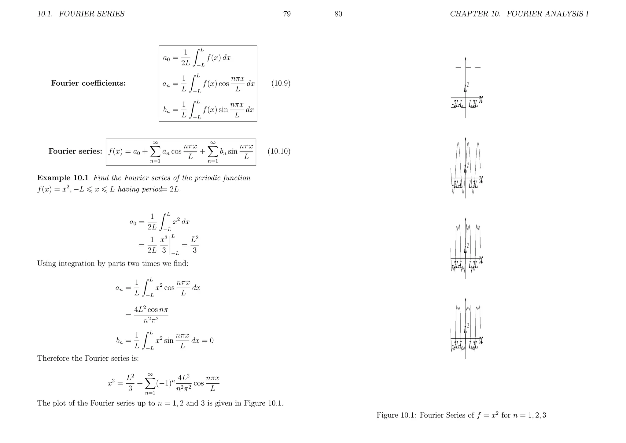
Theorem 10.2: Let f be continuous on [−L, L], f (L) = f (−L) and let f
be piecewise continuous. Then the Fourier coefficients of f satisfy:
∞
2a2 +
0
having period= 2L. Then evaluate the series at x = L.
a0 =
1
2L
a dx +
−L
1
2L
L
b dx =
0
a+b
2
L
1
L
f (x)2 dx
∞
f 2 (x) = a0 f (x) +
∞
L
f 2 (x) dx = a0
f (x) dx +
−L
∞
n=1
an cos nπx +
L
bn =
1
L
0
nπx
1
a cos
dx +
L
L
−L
0
a sin
−L
nπx
1
dx +
L
L
a L
nπx
=−
cos
L nπ
L
0
L
0
n=1
∞
L
an
f (x) cos
−L
nπx
bn
dx +
L
n=1
b sin
0
L
0
b−a
=
(1 − (−1)n )
nπ
Therefore the Fourier series is:
∞
a+b
b−a
nπx
+
[1 − (−1)n ] sin
f (x) =
2
nπ
L
n=1
a + b 2(b − a)
+
2
π
πx 1
3πx 1
5πx
+ sin
+ sin
+ ···
L
3
L
5
L
a+b
If we insert x = L in that series, we obtain f (L) =
. Thus the value at
2
discontinuity is the average of left and right limits. The summation of the
series up to n = 1, 5 and 9 is plotted on Figure 10.2.
=
f (x) sin
−L
1
1
1
= 1 + 4 + 4 + ···
4
n
2
3
n=1
2
(Hint: Use the Fourier series of f (x) = x on the interval −π < x < π)
Example 10.3 Find the sum of the series S =
nπx
dx
L
b L
nπx
−
cos
L nπ
L
−L
L
Using equation (10.9) to evaluate these integrals, we can obtain the result.
nπx
b cos
dx = 0
L
L
sin nπx .
L
nπx
nπx
+
bn f (x) sin
L
L
n=1
∞
1
an =
L
∞
n=1 bn
∞
an f (x) cos
n=1
L
(10.11)
−L
Proof: We can express f (x) as f (x) = a0 +
Now multiply both sides by f and integrate
−L
0
(a2 + b2 ) =
n
n
n=1
−L < x < 0
0<x<L
if
if
Parseval’s Identity
Evaluating the integrals in (10.9) for f (x) = x2 we obtain
π2
4(−1)n
and bn = 0 so
a0 = , a n =
3
n2
f (x) =
1
π2
1
− 4 cos x − cos 2x + cos 3x − · · ·
3
4
9
Using Parseval’s theorem, we have
sin
1
2π 4
1
+ 16 1 + 4 + 4 + · · ·
9
2
3
Therefore
1 π 4
x dx
π −π
2
= π4
5
=
nπx
d
L](https://image.slidesharecdn.com/258lecnot2-131215083806-phpapp02/75/258-lecnot2-46-2048.jpg)
![88
CHAPTER 11. FOURIER ANALYSIS II
Figure 11.1: Plots of Some Even and Odd Functions
Chapter 11
Fourier Analysis II
In this chapter, we will study more advanced properties of Fourier series. We
will find the even and odd periodic extensions of a given function, we will
express the series using complex notation and finally, we will extend the idea
of Fourier series to nonperiodic functions in the form of a Fourier integral.
As you can see in Figure 11.1, an even function is symmetric with respect
to y−axis, an odd function is symmetric with respect to origin.
Half Range Extensions: Let f be a function defined on [0, L]. If we want
to expand it in terms of sine and cosine functions, we can think of it as
periodic with period 2L. Now we need to define f on the interval [−L, 0].
There are infinitely many possibilities, but for simplicity, we are interested
in making f an even or an odd function. If we define f for negative x
values as f (x) = f (−x), we obtain the even periodic extension of f , which
is represented by a Fourier cosine series. If we define f for negative x values
as f (x) = −f (−x), we obtain the odd periodic extension of f , which is
represented by a Fourier sine series.
Half-Range Cosine Expansion: (or Fourier cosine series)
∞
f (x) = a0 +
11.1
n=1
Fourier Cosine and Sine Series
If f (−x) = f (x), f is an even function. If f (−x) = −f (x), f is an odd
function. We can easily see that, for functions:
even × even = even,
odd × odd = even,
even × odd = odd
For example |x|, x2 , x4 , cos x, cos nx, cosh x are even functions. x, x3 , sin x, sin nx, sinh x
are odd functions. ex is neither even nor odd.
L
L
If f is even:
f (x) dx
f (x) dx = 2
−L
L
If f is odd:
(11.1)
0
f (x) dx = 0
(11.2)
−L
Using the above equations, we can see that in the Fourier expansion of an
even function, bn = 0, and in the expansion of an odd function, an = 0. This
will cut our work in half if we can recognize the given function as odd or
even.
87
an cos
where a0 =
1
L
nπx
, (0 < x < L)
L
L
f (x) dx,
0
an =
2
L
L
f (x) cos
0
nπx
dx
L
(11.3)
(11.4)](https://image.slidesharecdn.com/258lecnot2-131215083806-phpapp02/75/258-lecnot2-49-2048.jpg)
![11.2. COMPLEX FOURIER SERIES
91
For n = 0 this integral is zero, so we have c0 = 0. For n = 0
cn =
−inx π
xe
−in
1
2π
π
−
−π
inπ
−π
1
2π
Therefore
CHAPTER 11. FOURIER ANALYSIS II
11.3
Fourier Integral Representation
−inx
e
dx
−in
πe−inπ + πe
−0
−in
1 einπ + e−inπ
cos nπ
=−
=−
in
2
in
i
n
= (−1)
n
=
92
In this section, we will apply the basic idea of the Fourier series to nonperiodic functions.
Consider a periodic function with period= 2L and its Fourier series. In
the limit L → ∞, the summation will be an integral, and f will be a nonperiodic function. Then we will obtain the Fourier integral representation:
∞
i
(−1)n einx ,
n
n=−∞
n=0
where
A(u) =
Note that we can obtain the real Fourier series from the complex one. If we
add nth and −nth terms we get
cos nx + i sin nx
cos(−nx) + i sin(−nx)
sin nx
i(−1)
+ i(−1)−n
= (−1)n+1
n
−n
n
B(u) =
n
∞
n+1 sin nx
(−1)
x=
n
n=1
1
π
1
π
∞
f (x) cos ux dx
(11.15)
f (x) sin ux dx
(11.16)
−∞
∞
−∞
Like the Fourier series, we have A(u) = 0 for odd functions and B(u) = 0 for
even functions.
Theorem 11.1: If f and f are piecewise continuous in every finite interval
∞
This is the real Fourier series.
|f | dx is convergent, then the Fourier integral of f converges to:
and if
−∞
Example 11.3 Find the complex Fourier series of f (x) = k
• f (x) if f is continuous at x.
π
1
ke−inx dx
2π −π
π
k e−inx
=
(n = 0)
2π −in −π
cn =
inπ
•
f (x+) + f (x−)
if f is discontinuous at x.
2
Example 11.4 Find the Fourier integral representation of
−inπ
k e −e
nπ
2i
k
=
sin nπ
nπ
=0
=
If n = 0 we have
(11.14)
0
∞
x=
[A(u) cos ux + B(u) sin ux] du
f (x) =
1
c0 =
2π
=k
f (x) =
π/2
0
if
if
|x| < 1
1 < |x|
Note that f is even therefore B(u) = 0
π
k dx
A(u) =
−π
∞
1
π
f (x) cos ux dx =
−∞
1
=
cos ux dx =
0
sin ux
u
1
π
1
=
0
1
−1
π
cos ux dx
2
sin u
u](https://image.slidesharecdn.com/258lecnot2-131215083806-phpapp02/75/258-lecnot2-51-2048.jpg)
![11.3. FOURIER INTEGRAL REPRESENTATION
93
Therefore, Fourier integral representation of f is
∞
f (x) =
0
sin u
cos ux du
u
94
CHAPTER 11. FOURIER ANALYSIS II
Exercises
For the following functions defined on 0 < x < L, find the half-range
cosine and half-range sine expansions:
Example 11.5 Prove the following formulas using two different methods:
eax
e cos bx dx = 2
(a cos bx + b sin bx)
a + b2
eax
eax sin bx dx = 2
(a sin bx − b cos bx)
a + b2
We can obtain the formulas using integration by parts, but this is the
long way. A better method is to express the integrals as a single complex
integral using eibx = cos bx + i sin bx, then evaluate it at one step, and then
separate the real and imaginary parts.
ax
Example 11.6 Find the Fourier integral representation of
f (x) =
−ex cos x
e−x cos x
if
if
x<0
0<x
This function is odd therefore A(u) = 0.
2 ∞ −x
1 ∞
f (x) sin ux dx =
e cos x sin ux dx
π −∞
π 0
2 ∞ −x sin(ux + x) + sin(ux − x)
e
dx
=
π 0
2
∞
1
e−x
=
[− sin(u + 1)x − (u + 1) cos(u + 1)x]
π 1 + (u + 1)2
0
∞
e−x
1
[− sin(u − 1)x − (u − 1) cos(u − 1)x]
+
π 1 + (u − 1)2
0
1
u−1
u+1
=
+
π 1 + (u + 1)2 1 + (u − 1)2
2 u3
=
π u4 + 4
B(u) =
So
f (x) =
2
π
∞
0
u3
sin ux du
+4
u4
1) f (x) =
2kx/L
2k(L − x)/L
if
if
0 < x < L/2
2) f (x) = ex
L/2 < x < L
3) f (x) = k
4) f (x) = x4
5) f (x) = cos 2x 0 < x < π
6) f (x) =
0
k
if
if
0 < x < L/2
L/2 < x < L
Find the complex Fourier series of the following functions:
7) f (x) =
0
1
if
if
−π < x < 0
0<x<π
9) f (x) = sin x
8) f (x) = x2 , −L < x < L
10) f (x) = cos 2x
Find the Fourier integral representations of the following functions:
π
π
cos x, |x| <
π − x, 0 < x < π
2
2
11) f (x) =
(f odd)
12) f (x) =
π
0,
π<x
0,
|x| >
2
13) f (x) =
e−x , 0 < x
ex , x < 0
π
0
14) f (x) =
Prove the following formulas. (Hint: Define a suitable
then find its Fourier integral representation.)
πx2 /2,
∞
2
cos ux
2
15)
1 − 2 sin u + cos u
du =
π/4,
u
u
u
0
0,
0,
x<0
∞
cos ux + u sin ux
16)
du =
π/2, x = 0
−x
1 + u2
0
πe , x > 0
if
if
0<x<1
Otherwise
function f and
0
x<1
x=1
1<x](https://image.slidesharecdn.com/258lecnot2-131215083806-phpapp02/75/258-lecnot2-52-2048.jpg)
![EXERCISES
95
f (x) =
16k
k
− 2
2
π
8k
π2
CHAPTER 11. FOURIER ANALYSIS II
i
i
9) f (x) = − eix + e−ix
2
2
1 2ix 1 −2ix
10) f (x) = e + e
2
2
Answers
1) f (x) =
96
1
1
2πx
6πx
+ 2 cos
+ ···
cos
2
2
L
6
L
1
1
1
πx
3πx
5πx
sin
− 2 sin
+ 2 sin
− ···
2
1
L
3
L
5
L
11) f (x) =
2
π
∞
2L
1
nπx
2) f (x) = (eL − 1) +
[(−1)n eL − 1] cos
2 + n2 π 2
L
L
L
n=1
∞
2nπ
nπx
[1 − (−1)n eL ] sin
2 + n2 π 2
L
L
f (x) =
n=1
∞
0
∞
12) f (x) =
2
π
∞
0
∞
3) f (x) = k
14) f (x) =
4k
f (x) =
π
0
3πx 1
5πx
πx 1
+ sin
+ sin
+ ···
sin
L
3
L
5
L
∞
L4
4) f (x) =
+ 8L4
(−1)n
5
n=1
∞
f (x) = 2L4
(−1)n+1
n=1
6
1
− 4 4
n2 π 2
nπ
cos
12
24
1
− 3 3+ 5 5
nπ
nπ
nπ
nπx
L
+
24
nπx
sin
5π5
n
L
5) f (x) = cos 2x
4
2
f (x) = −
sin x +
3π
π
6) f (x) =
f (x) =
k
2k
−
2
π
2k
π
∞
n=1
∞
n=1
∞
[1 − (−1)n ]
n=3
n
sin nx
n2 − 4
sin nπ
nπx
2
cos
n
L
cos nπ − cos nπ
nπx
2
sin
n
L
∞
1
i
[(−1)n − 1]einx , n = 0
7) f (x) = +
2 n=−∞ 2πn
8) f (x) =
L2 2L2
+ 2
3
π
∞
(−1)n inπx/L
e
, n=0
n2
n=−∞
cos
0
13) f (x) =
πu − sin πu
sin xu du
u2
πu
2
cos xu
du
1 − u2
cos xu
du
1 + u2
1 − cos u
u
sin ux +
sin u
cos ux du
u](https://image.slidesharecdn.com/258lecnot2-131215083806-phpapp02/75/258-lecnot2-53-2048.jpg)
![EXERCISES
105
Answers
1) u(x, t) = sin(2x) cos(4t)
∞
2) u(x, t) =
n=1
=
4
n3 π 3
[1 − (−1)n ] sin(nπx) cos(nπt)
1
8
sin(πx) cos(πt) +
sin(3πx) cos(3πt) + · · ·
π3
27
3) u(x, t) = 5 sin(πx) cos
∞
4) u(x, t) =
n=1
∞
5) u(x, t) =
n=1
=
6) u(x, t) =
πt
3
− 3 sin(2πx) cos
2πt
3
2hL2
nπa
nπx
sin
sin
cos
− a)
L
L
n2 π 2 a(L
nπct
L
4
[1 − (−1)n ] sin(nx) sin(nt)
n4 π
8
1
sin(πx) sin(πt) +
sin(3πx) sin(3πt) + · · ·
π
81
√
1
√ sin(πx) sin(2π 3t)
2π 3
∞
7) u(x, t) =
n=1
∞
8) u(x, t) =
n=1
0.4
nπ
sin
sin(nx) sin(nt)
3π
n
2
5
nπx
[1 − (−1)n ] sin
sin
n2 π 2
5
2nπt
5
106
CHAPTER 12. PARTIAL DIFFERENTIAL EQUATIONS](https://image.slidesharecdn.com/258lecnot2-131215083806-phpapp02/75/258-lecnot2-58-2048.jpg)

![EXERCISES
115
Answers
1) u(x, t) = sin 2x e−4t
2) u(x, t) = sin
∞
3) u(x, t) =
n=1
πx − 5 π2 t
2
e 4 − sin(πx) e−5π t
2
4L2
n2 π 2 kt
nπx
exp −
[1 − (−1)n ] sin
n3 π 3
L
L2
∞
4) u(x, t) =
2
π
2
+
[(−1)n − 1] cos nx e−n t
2 n=1 n2 π
5) u(x, t) = cos(0.3πx) e−0.27π
2t
∞
6) u(x, t) =
1
2
nπx
n2 π 2 kt
+
[1 − (−1)n ] cos
exp −
2 n=1 n2 π 2
L
L2
2
7) u(x, t) = 1 − x + e−π t sin πx −
2
π
∞
n=1
sin nπx −n2 π2 t
e
n
∞
8) u(x, t) =
=
Tx
2T
nπ
nπx −n2 π2 kt/L2
+
cos
sin
e
L
nπ
2
L
n=1
2T
Tx
−
L
π
9) u(x, y, t) = sin
πx
πy −2.32π2 t
sin
e
2
5
4T
10) u(x, y, t) = 2
π
Where Anm =
1
2πx −4π2 kt/L2
1
4πx −16π2 kt/L2
sin
e
− sin
e
+ ···
2
L
4
L
∞
∞
Anm sin
n=1 m=1
nπx
mπy −kπ2
sin
e
a
b
(1 − (−1)n ) (1 − (−1)m )
nm
2
n2
+m
a2
b2
t
116
CHAPTER 13. HEAT EQUATION](https://image.slidesharecdn.com/258lecnot2-131215083806-phpapp02/75/258-lecnot2-63-2048.jpg)
![14.1. RECTANGULAR COORDINATES
119
Superposition of these solutions give
CHAPTER 14. LAPLACE EQUATION
Example 14.1 Solve uxx + uyy = 0 on 0 < x < 2, 0 < y < 1, with
BC: u(0, y) = 0, u(2, y) = 0, u(x, 0) = 0, u(x, 1) = 1
∞
u(x, y) =
120
Bn sin
n=1
nπy
nπx
sinh
a
a
(14.9)
Using the steps above, we find
∞
We have only the fourth boundary condition left: y = b ⇒ u = f (x)
u(x, y) =
n=1
∞
nπb
nπx
sinh
= f (x)
u(x, b) =
Bn sin
a
a
n=1
(14.10)
nπb
2
=
a
a
a
f (x) sin
0
nπx
dx
a
Bn sinh
(14.11)
Remark: If two sides have nonzero BC, we can consider them as two separate problems having zero BC on 3 sides, find the solutions and then add
them to obtain the result, as you can see on Figure 14.2.
nπy
nπx
sinh
2
2
where
Obviously, Bn sinh nπb are the Fourier sine coefficients of f (x), so
a
Bn sinh
Bn sin
∞
u(x, y) =
n=1
2
nπx
dx
2
0
2[1 − (−1)n ]
Bn =
nπ sinh nπ
2
nπ
=
2
sin
2[1 − (−1)n ]
nπx
nπy
sin
sinh
nπ sinh nπ
2
2
2
You can see the solution on Figure 14.3 (up).
Example 14.2 Solve uxx + uyy = 0 on 0 < x < 1, 0 < y < 1, with
BC: u(x, 0) = 0, u(x, 1) = 0, u(0, y) = 0, u(1, y) = 3y(1 − y)
The solution satisfying the first three boundary conditions is:
∞
cn sinh(nπx) sin(nπy)
u(x, y) =
n=1
Inserting x = 1 and using the fourth boundary condition, we obtain
Figure 14.2: Nonzero Boundary Conditions on two sides
1
3y(1 − y) sin(nπy) dy
sinh(nπ) cn = 2
0
sinh(nπ) cn = 6 −
y cos nπy sin nπy y 2 cos nπy
2 cos nπy
2y sin nπy
+ 2 2 +
−
−
2π2
nπ
nπ
nπ
n
n3 π 3
cn =
12
u(x, y) = 3
π
∞
n=1
12[1 − (−1)n ]
n3 π 3 sinh(nπ)
[1 − (−1)n ]
sinh(nπx) sin(nπy)
n3 sinh(nπ)
Figure 14.3 (down) gives the plot.
1
0](https://image.slidesharecdn.com/258lecnot2-131215083806-phpapp02/75/258-lecnot2-65-2048.jpg)

We expect the solution to be periodic in θ with period 2π. Case 3 does
not satisfy this, so we eliminate this case.](https://image.slidesharecdn.com/258lecnot2-131215083806-phpapp02/75/258-lecnot2-66-2048.jpg)
![14.2. POLAR COORDINATES
123
In Case 1, we have to choose C = 0 for periodicity. Besides, ln r is
undefined at r = 0. So A = 0. Therefore the contribution of Case 1 is only
a constant.
In Case 2, r−p is undefined at r = 0, so we choose B = 0. The resulting
separated solution is:
124
CHAPTER 14. LAPLACE EQUATION
Example 14.3 Solve Laplace equation in the region 0
−1 if −π < θ < 0
BC: u(5, θ) =
1
if 0 < θ < π
r < 5, with
We know that the general solution in this case is
∞
un (r, θ) = rn (Cn cos nθ + Dn sin nθ)
rn (Cn cos nθ + Dn sin nθ)
u(r, θ) = C0 +
(14.18)
n=1
The boundary condition gives
Note that n must be an integer for periodicity.
After superposition, we obtain the general solution as
∞
5n (Cn cos nθ + Dn sin nθ) = f (θ)
u(5, θ) = C0 +
n=1
∞
rn (Cn cos nθ + Dn sin nθ)
u(r, θ) = C0 +
(14.19)
The Fourier coefficients of f are
n=1
The boundary condition is: u(a, θ) = f (θ), we can find Cn and Dn using the
Fourier expansion of f .
1
C0 =
2π
1
Cn = n
a π
1
Dn = n
a π
2
u(r, θ) =
π
π
f (θ) dθ
−π
π
f (θ) cos nθ dθ
(14.20)
−π
π
2
[1 − (−1)n ]
nπ5n
∞
[1 − (−1)n ]
n=1
r
5
n
sin nθ
n
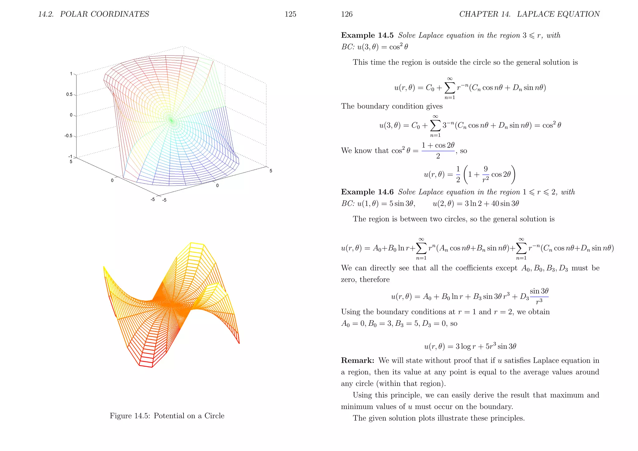
The solution is plotted on Figure 14.5 (up).
Example 14.4 Solve Laplace equation in the region 0
BC: u(2, θ) = sin(3θ)
f (θ) sin nθ dθ
−π
Remark: If the region is outside the circle, the same ideas apply. We have
to eliminate ln r because it is not finite at infinity. The only difference is that
we should have the negative powers of r, because they will be bounded as
r → ∞. So
r < 2, with
Inserting r = 2 in the solution
∞
rn (Cn cos nθ + Dn sin nθ)
u(r, θ) = C0 +
n=1
we obtain
∞
u(r, θ) = C0 +
C0 = 0, Cn = 0, Dn =
r
−n
(Cn cos nθ + Dn sin nθ)
(14.21)
n=1
Remark: If we have a region between two circles as a < r < b, we need
both the positive and negative powers of r as well as the logarithmic term.
∞
2n (Cn cos nθ + Dn sin nθ) = sin 3θ
u(2, θ) = C0 +
n=1
We can easily see that the only nonzero Fourier coefficient is D3
23 D3 = 1
⇒
D3 =
1 3
r sin 3θ
8
The solution is plotted on Figure 14.5 (down).
u(r, θ) =
1
8](https://image.slidesharecdn.com/258lecnot2-131215083806-phpapp02/75/258-lecnot2-67-2048.jpg)
![To the Student
If you have reached this point after solving all (or most) of the exercises,
you must have covered a lot of ground. But there’s no end to differential
equations. This was just a brief introduction. For further study, you may
consult the books listed in the references.
[6, 8] and [9] are big and useful books that contain all topics covered here
and many other ones besides.
For ordinary differential equations, [2, 11, 12, 14] give a complete treatment with a large number of exercises.
For partial differential equations, [1] and [7] are good introductory books
that illustrate main ideas.
Detailed information on Fourier Series can be found on [3].
There are many aspects of differential equations that we did not even
touch in this book.
For a history of this subject, you may consult [13].
For nonlinear equations and dynamical systems, which is a vast subject
requiring another book even for the introduction, [10] and [15] will be a good
starting point.
For numerical methods, you may read the relevant chapters of [4] and [5].
129](https://image.slidesharecdn.com/258lecnot2-131215083806-phpapp02/75/258-lecnot2-70-2048.jpg)
![132
REFERENCES
[11] Rainville, E.D., Bedient, P.E. and Bedient, R.E. Elementary Differential
Equations, 8th edition. Prentice Hall, 1997.
[12] Ross, S.L. Introduction to Ordinary Differential Equations, 4th edition.
Wiley, 1989.
References
[13] Simmons, G.F. Differential Equations with Applications and Historical
Notes, 2nd edition. McGraw–Hill, 1991.
[1] Asmar, N.H. Partial Differential Equations and Boundary Value Problems. Prentice Hall, 2000.
[2] Boyce, W.E. and DiPrima, R.C. Elementary Differential Equations and
Boundary Value Problems, 6th edition. Wiley, 1997.
[3] Churchill, R.V. and Brown, J.W. Fourier Series and Boundary Value
Problems, 6th edition. McGraw–Hill, 2000.
[4] Fausett, L.V. Numerical Methods: Algorithms and Applications. Prentice Hall, 2003.
[5] Gerald, C.F. and Wheatley, P.O. Applied Numerical Analysis, 7th edition. Prentice Hall, 2004.
[6] Greenberg, M.D. Advanced Engineering Mathematics, 2nd edition. Prentice Hall, 1998.
[7] Keane, M.K. A Very Applied First Course in Partial Differential Equations. Prentice Hall, 2002.
[8] Kreyszig, E. Advanced Engineering Mathematics, 8th edition. Wiley,
1998.
[9] O’Neil, P.V. Advanced Engineering Mathematics, 5th edition. Thomson,
2003.
[10] Perko, L. Differential Equations and Dynamical Systems, 3rd edition.
Springer, 2001.
131
[14] Trench, W.F. Elementary Differential Equations with Boundary Value
Problems. Brooks/Cole, 2001.
[15] Williamson, R.E. Introduction to Differential Equations and Dynamical
Systems, 2nd edition. McGraw–Hill, 2000.](https://image.slidesharecdn.com/258lecnot2-131215083806-phpapp02/75/258-lecnot2-71-2048.jpg)

Here are the key steps to solve this separable differential equation: 1) Separate the variables: dy/dx = (1-y^2) 2) Integrate both sides: ∫ dy/(1-y^2) = ∫ dx 3) Evaluate the integrals: arctan(y) = x + C 4) Take the inverse tangent of both sides: y = tan(x + C) This is the general solution. 1.4 Transformations We can transform a differential equation into a separable one using the following techniques: So the general solution is: y = tan(x + C) 1. Change of variables: