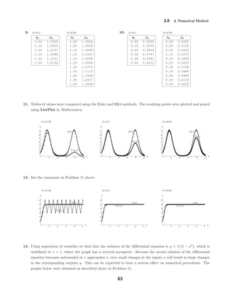
The document contains 40 multi-part exercises involving analyzing first-order differential equations and their solution curves based on direction fields and phase portraits. The exercises involve identifying critical points, determining stability of critical points, classifying regions where solution curves are increasing or decreasing, sketching phase portraits, and determining limiting behavior of solutions.

1. -3 -2 -1 1 2 3
x
-3
-2
-1
1
2
3
y
-10 -5 0 5 10
-5
0
5
10
x
y
-4 -2 0 2 4
-2
0
2
4
x
y
-4 -2 0 2 4
-4
-2
0
2
4
x
y
-4 -2 0 2 4
-2
0
2
4
x
y
-4 -2 0 2 4
-2
0
2
4
x
y
22 First-Order Differential Equations
EXERCISES 2.1
Solution Curves Without the Solution
1. 2.
3. 4.
5. 6.
22

2. -4 -2 0 2 4
-4
-2
0
2
4
x
y
-4 -2 0 2 4
-2
0
2
4
x
y
-4 -2 0 2 4
-2
0
2
4
x
y
-4 -2 0 2 4
-2
0
2
4
x
y
-4 -2 0 2 4
-2
0
2
4
x
y
-4 -2 0 2 4
-2
0
2
4
x
y
-3 -2 -1 0 1 2 3
-3
-2
-1
0
1
2
3
x
y
-4 -2 0 2 4
-4
-2
0
2
4
x
y
2.1 Solution Curves Without the Solution
7. 8.
9. 10.
11. 12.
13. 14.
23

3. -3 -2 -1 1 2 3 x
-3
-2
-1
1
2
3
y
-2 -1 1 2 x
-2
-1
1
2
y
-3 -2 -1 0 1 2 3
-3
-2
-1
0
1
2
3
x
y
2.1 Solution Curves Without the Solution
15. (a) The isoclines have the form y = −x + c, which are straight
lines with slope −1.
(b) The isoclines have the form x2
+ y2
= c, which are circles
centered at the origin.
16. (a) When x = 0 or y = 4, dy/dx = −2 so the lineal elements have slope −2. When y = 3 or y = 5, dy/dx = x−2,
so the lineal elements at (x, 3) and (x, 5) have slopes x − 2.
(b) At (0, y0) the solution curve is headed down. If y → ∞ as x increases, the graph must eventually turn
around and head up, but while heading up it can never cross y = 4 where a tangent line to a solution curve
must have slope −2. Thus, y cannot approach ∞ as x approaches ∞.
17. When y < 1
2 x2
, y = x2
− 2y is positive and the portions of solution
curves “outside” the nullcline parabola are increasing. When y > 1
2 x2
,
y = x2
−2y is negative and the portions of the solution curves “inside” the
nullcline parabola are decreasing.
18. (a) Any horizontal lineal element should be at a point on a nullcline. In Problem 1 the nullclines are x2
−y2
= 0
or y = ±x. In Problem 3 the nullclines are 1 − xy = 0 or y = 1/x. In Problem 4 the nullclines are
(sin x) cos y = 0 or x = nπ and y = π/2 + nπ, where n is an integer. The graphs on the next page show the
nullclines for the differential equations in Problems 1, 3, and 4 superimposed on the corresponding direction
field.
24

4. -3 -2 -1 0 1 2 3
Problem 1
-3
-2
-1
0
1
2
3
x
y
-4 -2 0 2 4
Problem 3
-4
-2
0
2
4
x
y
-4 -2 0 2 4
Problem 4
-4
-2
0
2
4
x
y
-1
0
1
1 2
x
5
4
3
2
1
y
1 2-1-2
x
1
y
1 2-1-2
x
-1
y
1 2
x
-5
-4
-3
-2
-1
y
-1
0
1
1 2
x
5
4
3
2
1
y
1 2-1-2
x
1
y
1 2-1-2
x
-1
y
-1-2
x
-5
-4
-3
-2
-1
y
2.1 Solution Curves Without the Solution
(b) An autonomous first-order differential equation has the form y = f(y). Nullclines have the form y = c
where f(c) = 0. These are the graphs of the equilibrium solutions of the differential equation.
19. Writing the differential equation in the form dy/dx = y(1 − y)(1 + y) we see that critical points
are located at y = −1, y = 0, and y = 1. The phase portrait is shown at the right.
(a) (b)
(c) (d)
20. Writing the differential equation in the form dy/dx = y2
(1 − y)(1 + y) we see that critical points
are located at y = −1, y = 0, and y = 1. The phase portrait is shown at the right.
(a) (b)
(c) (d)
25

5. 0
3
0
1
2
-2
5
2.1 Solution Curves Without the Solution
21. Solving y2
− 3y = y(y − 3) = 0 we obtain the critical points 0 and 3. From the phase portrait we
see that 0 is asymptotically stable (attractor) and 3 is unstable (repeller).
22. Solving y2
− y3
= y2
(1 − y) = 0 we obtain the critical points 0 and 1. From the phase portrait we
see that 1 is asymptotically stable (attractor) and 0 is semi-stable.
23. Solving (y − 2)4
= 0 we obtain the critical point 2. From the phase portrait we see that 2 is
semi-stable.
24. Solving 10 + 3y − y2
= (5 − y)(2 + y) = 0 we obtain the critical points −2 and 5. From the phase
portrait we see that 5 is asymptotically stable (attractor) and −2 is unstable (repeller).
26

6. -2
0
2
0
2
4
-1
0
-2
0
ln 9
2.1 Solution Curves Without the Solution
25. Solving y2
(4−y2
) = y2
(2−y)(2+y) = 0 we obtain the critical points −2, 0, and 2. From the phase
portrait we see that 2 is asymptotically stable (attractor), 0 is semi-stable, and −2 is unstable
(repeller).
26. Solving y(2 − y)(4 − y) = 0 we obtain the critical points 0, 2, and 4. From the phase portrait we
see that 2 is asymptotically stable (attractor) and 0 and 4 are unstable (repellers).
27. Solving y ln(y + 2) = 0 we obtain the critical points −1 and 0. From the phase portrait we see that
−1 is asymptotically stable (attractor) and 0 is unstable (repeller).
28. Solving yey
−9y = y(ey
−9) = 0 we obtain the critical points 0 and ln 9. From the phase portrait
we see that 0 is asymptotically stable (attractor) and ln 9 is unstable (repeller).
29. The critical points are 0 and c because the graph of f(y) is 0 at these points. Since f(y) > 0 for y < 0 and
y > c, the graph of the solution is increasing on (−∞, 0) and (c, ∞). Since f(y) < 0 for 0 < y < c, the graph of
the solution is decreasing on (0, c).
27

7. 0
c
x
c
y
-2.2
0.5
1.7
-2 -1 1 2
x
-2
-1
1
2
y
Π Π
2
Π
2
Π
y
-1
1
0
Π
2
Π
2
2.1 Solution Curves Without the Solution
30. The critical points are approximately at −2, 2, 0.5, and 1.7. Since f(y) > 0 for y < −2.2 and 0.5 < y < 1.7, the
graph of the solution is increasing on (−∞, −2.2) and (0.5, 1.7). Since f(y) < 0 for −2.2 < y < 0.5 and y > 1.7,
the graph is decreasing on (−2.2, 0.5) and (1.7, ∞).
31. From the graphs of z = π/2 and z = sin y we see that
(π/2)y − sin y = 0 has only three solutions. By inspection
we see that the critical points are −π/2, 0, and π/2.
From the graph at the right we see that
2
π
y − sin y
< 0 for y < −π/2
> 0 for y > π/2
2
π
y − sin y
> 0 for − π/2 < y < 0
< 0 for 0 < y < π/2.
This enables us to construct the phase portrait shown at the right. From this portrait we see that π/2 and
−π/2 are unstable (repellers), and 0 is asymptotically stable (attractor).
32. For dy/dx = 0 every real number is a critical point, and hence all critical points are nonisolated.
33. Recall that for dy/dx = f(y) we are assuming that f and f are continuous functions of y on some interval
I. Now suppose that the graph of a nonconstant solution of the differential equation crosses the line y = c.
If the point of intersection is taken as an initial condition we have two distinct solutions of the initial-value
problem. This violates uniqueness, so the graph of any nonconstant solution must lie entirely on one side of
any equilibrium solution. Since f is continuous it can only change signs at a point where it is 0. But this is a
critical point. Thus, f(y) is completely positive or completely negative in each region Ri. If y(x) is oscillatory
28

8. x
y
-5 5
-5
5
0
b
a
mg
k
2.1 Solution Curves Without the Solution
or has a relative extremum, then it must have a horizontal tangent line at some point (x0, y0). In this case y0
would be a critical point of the differential equation, but we saw above that the graph of a nonconstant solution
cannot intersect the graph of the equilibrium solution y = y0.
34. By Problem 33, a solution y(x) of dy/dx = f(y) cannot have relative extrema and hence must be monotone.
Since y (x) = f(y) > 0, y(x) is monotone increasing, and since y(x) is bounded above by c2, limx→∞ y(x) = L,
where L ≤ c2. We want to show that L = c2. Since L is a horizontal asymptote of y(x), limx→∞ y (x) = 0.
Using the fact that f(y) is continuous we have
f(L) = f( lim
x→∞
y(x)) = lim
x→∞
f(y(x)) = lim
x→∞
y (x) = 0.
But then L is a critical point of f. Since c1 < L ≤ c2, and f has no critical points between c1 and c2, L = c2.
35. Assuming the existence of the second derivative, points of inflection of y(x) occur where y (x) = 0. From
dy/dx = f(y) we have d2
y/dx2
= f (y) dy/dx. Thus, the y-coordinate of a point of inflection can be located by
solving f (y) = 0. (Points where dy/dx = 0 correspond to constant solutions of the differential equation.)
36. Solving y2
− y − 6 = (y − 3)(y + 2) = 0 we see that 3 and −2 are critical points.
Now d2
y/dx2
= (2y−1) dy/dx = (2y−1)(y−3)(y+2), so the only possible point
of inflection is at y = 1
2 , although the concavity of solutions can be different on
either side of y = −2 and y = 3. Since y (x) < 0 for y < −2 and 1
2 < y < 3,
and y (x) > 0 for −2 < y < 1
2 and y > 3, we see that solution curves are
concave down for y < −2 and 1
2 < y < 3 and concave up for −2 < y < 1
2 and
y > 3. Points of inflection of solutions of autonomous differential equations will
have the same y-coordinates because between critical points they are horizontal
translates of each other.
37. If (1) in the text has no critical points it has no constant solutions. The solutions have neither an upper nor
lower bound. Since solutions are monotonic, every solution assumes all real values.
38. The critical points are 0 and b/a. From the phase portrait we see that 0 is an attractor and b/a
is a repeller. Thus, if an initial population satisfies P0 > b/a, the population becomes unbounded
as t increases, most probably in finite time, i.e. P(t) → ∞ as t → T. If 0 < P0 < b/a, then the
population eventually dies out, that is, P(t) → 0 as t → ∞. Since population P > 0 we do not
consider the case P0 < 0.
39. (a) Writing the differential equation in the form
dv
dt
=
k
m
mg
k
− v
we see that a critical point is mg/k.
From the phase portrait we see that mg/k is an asymptotically stable critical
point. Thus, limt→∞ v = mg/k.
29

9. mg
k
Α
Β
Α
2.1 Solution Curves Without the Solution
(b) Writing the differential equation in the form
dv
dt
=
k
m
mg
k
− v2
=
k
m
mg
k
− v
mg
k
+ v
we see that the only physically meaningful critical point is mg/k.
From the phase portrait we see that mg/k is an asymptotically stable
critical point. Thus, limt→∞ v = mg/k.
40. (a) From the phase portrait we see that critical points are α and β. Let X(0) = X0. If X0 < α,
we see that X → α as t → ∞. If α < X0 < β, we see that X → α as t → ∞. If X0 > β, we see
that X(t) increases in an unbounded manner, but more specific behavior of X(t) as t → ∞ is
not known.
(b) When α = β the phase portrait is as shown. If X0 < α, then X(t) → α as t → ∞. If X0 > α,
then X(t) increases in an unbounded manner. This could happen in a finite amount of time.
That is, the phase portrait does not indicate that X becomes unbounded as t → ∞.
(c) When k = 1 and α = β the differential equation is dX/dt = (α − X)2
. For X(t) = α − 1/(t + c) we have
dX/dt = 1/(t + c)2
and
(α − X)2
= α − α −
1
t + c
2
=
1
(t + c)2
=
dX
dt
.
For X(0) = α/2 we obtain
X(t) = α −
1
t + 2/α
.
For X(0) = 2α we obtain
X(t) = α −
1
t − 1/α
.
30

10. t
X
−2/α
α
α/2 t
X
1/α
α
2α
2.2 Separable Variables
For X0 > α, X(t) increases without bound up to t = 1/α. For t > 1/α, X(t) increases but X → α as
t → ∞
EXERCISES 2.2
Separable Variables
In many of the following problems we will encounter an expression of the form ln |g(y)| = f(x)+c. To solve for g(y)
we exponentiate both sides of the equation. This yields |g(y)| = ef(x)+c
= ec
ef(x)
which implies g(y) = ±ec
ef(x)
.
Letting c1 = ±ec
we obtain g(y) = c1ef(x)
.
1. From dy = sin 5x dx we obtain y = −1
5 cos 5x + c.
2. From dy = (x + 1)2
dx we obtain y = 1
3 (x + 1)3
+ c.
3. From dy = −e−3x
dx we obtain y = 1
3 e−3x
+ c.
4. From
1
(y − 1)2
dy = dx we obtain −
1
y − 1
= x + c or y = 1 −
1
x + c
.
5. From
1
y
dy =
4
x
dx we obtain ln |y| = 4 ln |x| + c or y = c1x4
.
6. From
1
y2
dy = −2x dx we obtain −
1
y
= −x2
+ c or y =
1
x2 + c1
.
7. From e−2y
dy = e3x
dx we obtain 3e−2y
+ 2e3x
= c.
8. From yey
dy = e−x
+ e−3x
dx we obtain yey
− ey
+ e−x
+
1
3
e−3x
= c.
9. From y + 2 +
1
y
dy = x2
ln x dx we obtain
y2
2
+ 2y + ln |y| =
x3
3
ln |x| −
1
9
x3
+ c.
10. From
1
(2y + 3)2
dy =
1
(4x + 5)2
dx we obtain
2
2y + 3
=
1
4x + 5
+ c.
11. From
1
csc y
dy = −
1
sec2 x
dx or sin y dy = − cos2
x dx = −1
2 (1 + cos 2x) dx we obtain
− cos y = −1
2 x − 1
4 sin 2x + c or 4 cos y = 2x + sin 2x + c1.
12. From 2y dy = −
sin 3x
cos3 3x
dx or 2y dy = − tan 3x sec2
3x dx we obtain y2
= −1
6 sec2
3x + c.
31

11. 2.2 Separable Variables
13. From
ey
(ey + 1)
2 dy =
−ex
(ex + 1)
3 dx we obtain − (ey
+ 1)
−1
= 1
2 (ex
+ 1)
−2
+ c.
14. From
y
(1 + y2)
1/2
dy =
x
(1 + x2)
1/2
dx we obtain 1 + y2 1/2
= 1 + x2 1/2
+ c.
15. From
1
S
dS = k dr we obtain S = cekr
.
16. From
1
Q − 70
dQ = k dt we obtain ln |Q − 70| = kt + c or Q − 70 = c1ekt
.
17. From
1
P − P2
dP =
1
P
+
1
1 − P
dP = dt we obtain ln |P| − ln |1 − P| = t + c so that ln
P
1 − P
= t + c or
P
1 − P
= c1et
. Solving for P we have P =
c1et
1 + c1et
.
18. From
1
N
dN = tet+2
− 1 dt we obtain ln |N| = tet+2
− et+2
− t + c or N = c1etet+2
−et+2
−t
.
19. From
y − 2
y + 3
dy =
x − 1
x + 4
dx or 1 −
5
y + 3
dy = 1 −
5
x + 4
dx we obtain y −5 ln |y +3| = x−5 ln |x+4|+c
or
x + 4
y + 3
5
= c1ex−y
.
20. From
y + 1
y − 1
dy =
x + 2
x − 3
dx or 1 +
2
y − 1
dy = 1 +
5
x − 3
dx we obtain y +2 ln |y −1| = x+5 ln |x−3|+c
or
(y − 1)2
(x − 3)5
= c1ex−y
.
21. From x dx =
1
1 − y2
dy we obtain 1
2 x2
= sin−1
y + c or y = sin
x2
2
+ c1 .
22. From
1
y2
dy =
1
ex + e−x
dx =
ex
(ex)2 + 1
dx we obtain −
1
y
= tan−1
ex
+ c or y = −
1
tan−1
ex + c
.
23. From
1
x2 + 1
dx = 4 dt we obtain tan−1
x = 4t + c. Using x(π/4) = 1 we find c = −3π/4. The solution of the
initial-value problem is tan−1
x = 4t −
3π
4
or x = tan 4t −
3π
4
.
24. From
1
y2 − 1
dy =
1
x2 − 1
dx or
1
2
1
y − 1
−
1
y + 1
dy =
1
2
1
x − 1
−
1
x + 1
dx we obtain
ln |y − 1| − ln |y + 1| = ln |x − 1| − ln |x + 1| + ln c or
y − 1
y + 1
=
c(x − 1)
x + 1
. Using y(2) = 2 we find
c = 1. A solution of the initial-value problem is
y − 1
y + 1
=
x − 1
x + 1
or y = x.
25. From
1
y
dy =
1 − x
x2
dx =
1
x2
−
1
x
dx we obtain ln |y| = −
1
x
− ln |x| = c or xy = c1e−1/x
. Using y(−1) = −1
we find c1 = e−1
. The solution of the initial-value problem is xy = e−1−1/x
or y = e−(1+1/x)
/x.
26. From
1
1 − 2y
dy = dt we obtain −1
2 ln |1 − 2y| = t + c or 1 − 2y = c1e−2t
. Using y(0) = 5/2 we find c1 = −4.
The solution of the initial-value problem is 1 − 2y = −4e−2t
or y = 2e−2t
+ 1
2 .
27. Separating variables and integrating we obtain
dx
√
1 − x2
−
dy
1 − y2
= 0 and sin−1
x − sin−1
y = c.
32

12. 2.2 Separable Variables
Setting x = 0 and y =
√
3/2 we obtain c = −π/3. Thus, an implicit solution of the initial-value problem is
sin−1
x − sin−1
y = π/3. Solving for y and using an addition formula from trigonometry, we get
y = sin sin−1
x +
π
3
= x cos
π
3
+ 1 − x2 sin
π
3
=
x
2
+
√
3
√
1 − x2
2
.
28. From
1
1 + (2y)2
dy =
−x
1 + (x2)
2 dx we obtain
1
2
tan−1
2y = −
1
2
tan−1
x2
+ c or tan−1
2y + tan−1
x2
= c1.
Using y(1) = 0 we find c1 = π/4. Thus, an implicit solution of the initial-value problem is
tan−1
2y + tan−1
x2
= π/4 . Solving for y and using a trigonometric identity we get
2y = tan
π
4
− tan−1
x2
y =
1
2
tan
π
4
− tan−1
x2
=
1
2
tan π
4 − tan(tan−1
x2
)
1 + tan π
4 tan(tan−1
x2)
=
1
2
1 − x2
1 + x2
.
29. (a) The equilibrium solutions y(x) = 2 and y(x) = −2 satisfy the initial conditions y(0) = 2 and y(0) = −2,
respectively. Setting x = 1
4 and y = 1 in y = 2(1 + ce4x
)/(1 − ce4x
) we obtain
1 = 2
1 + ce
1 − ce
, 1 − ce = 2 + 2ce, −1 = 3ce, and c = −
1
3e
.
The solution of the corresponding initial-value problem is
y = 2
1 − 1
3 e4x−1
1 + 1
3 e4x−1
= 2
3 − e4x−1
3 + e4x−1
.
(b) Separating variables and integrating yields
1
4
ln |y − 2| −
1
4
ln |y + 2| + ln c1 = x
ln |y − 2| − ln |y + 2| + ln c = 4x
ln
c(y − 2)
y + 2
= 4x
c
y − 2
y + 2
= e4x
.
Solving for y we get y = 2(c + e4x
)/(c − e4x
). The initial condition y(0) = −2 implies
2(c + 1)/(c − 1) = −2 which yields c = 0 and y(x) = −2. The initial condition y(0) = 2 does not
correspond to a value of c, and it must simply be recognized that y(x) = 2 is a solution of the initial-value
problem. Setting x = 1
4 and y = 1 in y = 2(c + e4x
)/(c − e4x
) leads to c = −3e. Thus, a solution of the
initial-value problem is
y = 2
−3e + e4x
−3e − e4x
= 2
3 − e4x−1
3 + e4x−1
.
30. Separating variables, we have
dy
y2 − y
=
dx
x
or
dy
y(y − 1)
= ln |x| + c.
33

13. -0.004-0.002 0.002 0.004
x
0.97
0.98
1
1.01
y
2.2 Separable Variables
Using partial fractions, we obtain
1
y − 1
−
1
y
dy = ln |x| + c
ln |y − 1| − ln |y| = ln |x| + c
ln
y − 1
xy
= c
y − 1
xy
= ec
= c1.
Solving for y we get y = 1/(1 − c1x). We note by inspection that y = 0 is a singular solution of the differential
equation.
(a) Setting x = 0 and y = 1 we have 1 = 1/(1 − 0), which is true for all values of c1. Thus, solutions passing
through (0, 1) are y = 1/(1 − c1x).
(b) Setting x = 0 and y = 0 in y = 1/(1 − c1x) we get 0 = 1. Thus, the only solution passing through (0, 0) is
y = 0.
(c) Setting x = 1
2 and y = 1
2 we have 1
2 = 1/(1 − 1
2 c1), so c1 = −2 and y = 1/(1 + 2x).
(d) Setting x = 2 and y = 1
4 we have 1
4 = 1/(1 − 2c1), so c1 = −3
2 and y = 1/(1 + 3
2 x) = 2/(2 + 3x).
31. Singular solutions of dy/dx = x 1 − y2 are y = −1 and y = 1. A singular solution of
(ex
+ e−x
)dy/dx = y2
is y = 0.
32. Differentiating ln(x2
+ 10) + csc y = c we get
2x
x2 + 10
− csc y cot y
dy
dx
= 0,
2x
x2 + 10
−
1
sin y
·
cos y
sin y
dy
dx
= 0,
or
2x sin2
y dx − (x2
+ 10) cos y dy = 0.
Writing the differential equation in the form
dy
dx
=
2x sin2
y
(x2 + 10) cos y
we see that singular solutions occur when sin2
y = 0, or y = kπ, where k is an integer.
33. The singular solution y = 1 satisfies the initial-value problem.
34

14. -0.004-0.002 0.002 0.004
x
0.98
0.99
1.01
1.02
y
-0.004-0.002 0.002 0.004
x
0.9996
0.9998
1.0002
1.0004
y
-0.004-0.002 0.002 0.004
x
0.9996
0.9998
1.0002
1.0004
y
2.2 Separable Variables
34. Separating variables we obtain
dy
(y − 1)2
= dx. Then
−
1
y − 1
= x + c and y =
x + c − 1
x + c
.
Setting x = 0 and y = 1.01 we obtain c = −100. The solution is
y =
x − 101
x − 100
.
35. Separating variables we obtain
dy
(y − 1)2 + 0.01
= dx. Then
10 tan−1
10(y − 1) = x + c and y = 1 +
1
10
tan
x + c
10
.
Setting x = 0 and y = 1 we obtain c = 0. The solution is
y = 1 +
1
10
tan
x
10
.
36. Separating variables we obtain
dy
(y − 1)2 − 0.01
= dx. Then, from (11) in
this section of the manual with u = y − 1 and a = 1
10 , we get
5 ln
10y − 11
10y − 9
= x + c.
Setting x = 0 and y = 1 we obtain c = 5 ln 1 = 0. The solution is
5 ln
10y − 11
10y − 9
= x.
Solving for y we obtain
y =
11 + 9ex/5
10 + 10ex/5
.
Alternatively, we can use the fact that
dy
(y − 1)2 − 0.01
= −
1
0.1
tanh−1 y − 1
0.1
= −10 tanh−1
10(y − 1).
(We use the inverse hyperbolic tangent because |y − 1| < 0.1 or 0.9 < y < 1.1. This follows from the initial
condition y(0) = 1.) Solving the above equation for y we get y = 1 + 0.1 tanh(x/10).
37. Separating variables, we have
dy
y − y3
=
dy
y(1 − y)(1 + y)
=
1
y
+
1/2
1 − y
−
1/2
1 + y
dy = dx.
Integrating, we get
ln |y| −
1
2
ln |1 − y| −
1
2
ln |1 + y| = x + c.
35

15. 1 2 3 4 5 x
-4
-2
2
4
y
-4 -2 2 4 x
-4
-2
2
4
y
-4 -2 2 4 x
-4
-2
2
4
y
1 2 3 4 5 x
-4
-2
2
4
y
-4 -2 2 4 x
-2
2
4
6
8
y
3
-1 1 2 3 4 5 x
-2
2
4
6
8
y
2.2 Separable Variables
When y > 1, this becomes
ln y −
1
2
ln(y − 1) −
1
2
ln(y + 1) = ln
y
y2 − 1
= x + c.
Letting x = 0 and y = 2 we find c = ln(2/
√
3 ). Solving for y we get y1(x) = 2ex
/
√
4e2x − 3 , where x > ln(
√
3/2).
When 0 < y < 1 we have
ln y −
1
2
ln(1 − y) −
1
2
ln(1 + y) = ln
y
1 − y2
= x + c.
Letting x = 0 and y = 1
2 we find c = ln(1/
√
3 ). Solving for y we get y2(x) = ex
/
√
e2x + 3 , where −∞ < x < ∞.
When −1 < y < 0 we have
ln(−y) −
1
2
ln(1 − y) −
1
2
ln(1 + y) = ln
−y
1 − y2
= x + c.
Letting x = 0 and y = −1
2 we find c = ln(1/
√
3 ). Solving for y we get y3(x) = −ex
/
√
e2x + 3 , where
−∞ < x < ∞.
When y < −1 we have
ln(−y) −
1
2
ln(1 − y) −
1
2
ln(−1 − y) = ln
−y
y2 − 1
= x + c.
Letting x = 0 and y = −2 we find c = ln(2/
√
3 ). Solving for y we get y4(x) = −2ex
/
√
4e2x − 3 , where
x > ln(
√
3/2).
38. (a) The second derivative of y is
d2
y
dx2
= −
dy/dx
(y − 1)2
= −
1/(y − 3)
(y − 3)2
= −
1
(y − 3)3
.
The solution curve is concave down when d2
y/dx2
< 0 or y > 3, and
concave up when d2
y/dx2
> 0 or y < 3. From the phase portrait we
see that the solution curve is decreasing when y < 3 and increasing
when y > 3.
(b) Separating variables and integrating we obtain
(y − 3) dy = dx
1
2
y2
− 3y = x + c
y2
− 6y + 9 = 2x + c1
(y − 3)2
= 2x + c1
y = 3 ±
√
2x + c1 .
36

16. -5 -4 -3 -2 -1 1 2 x
-5
-4
-3
-2
-1
1
2
y
-2 -1.5 -1 -0.5 x
-2
-1
1
2
y
2.2 Separable Variables
The initial condition dictates whether to use the plus or minus sign.
When y1(0) = 4 we have c1 = 1 and y1(x) = 3 +
√
2x + 1 .
When y2(0) = 2 we have c1 = 1 and y2(x) = 3 −
√
2x + 1 .
When y3(1) = 2 we have c1 = −1 and y3(x) = 3 −
√
2x − 1 .
When y4(−1) = 4 we have c1 = 3 and y4(x) = 3 +
√
2x + 3 .
39. (a) Separating variables we have 2y dy = (2x + 1)dx. Integrating gives y2
= x2
+ x + c. When y(−2) = −1 we
find c = −1, so y2
= x2
+ x − 1 and y = −
√
x2 + x − 1 . The negative square root is chosen because of the
initial condition.
(b) From the figure, the largest interval of definition appears to be
approximately (−∞, −1.65).
(c) Solving x2
+ x − 1 = 0 we get x = −1
2 ± 1
2
√
5 , so the largest interval of definition is (−∞, −1
2 − 1
2
√
5 ).
The right-hand endpoint of the interval is excluded because y = −
√
x2 + x − 1 is not differentiable at this
point.
40. (a) From Problem 7 the general solution is 3e−2y
+2e3x
= c. When y(0) = 0 we find c = 5, so 3e−2y
+2e3x
= 5.
Solving for y we get y = −1
2 ln 1
3 (5 − 2e3x
).
(b) The interval of definition appears to be approximately (−∞, 0.3).
(c) Solving 1
3 (5 − 2e3x
) = 0 we get x = 1
3 ln(5
2 ), so the exact interval of definition is (−∞, 1
3 ln 5
2 ).
41. (a) While y2(x) = −
√
25 − x2 is defined at x = −5 and x = 5, y2(x) is not defined at these values, and so the
interval of definition is the open interval (−5, 5).
(b) At any point on the x-axis the derivative of y(x) is undefined, so no solution curve can cross the x-axis.
Since −x/y is not defined when y = 0, the initial-value problem has no solution.
42. (a) Separating variables and integrating we obtain x2
− y2
= c. For c = 0 the graph is a hyperbola centered at
the origin. All four initial conditions imply c = 0 and y = ±x. Since the differential equation is not defined
for y = 0, solutions are y = ±x, x < 0 and y = ±x, x > 0. The solution for y(a) = a is y = x, x > 0; for
y(a) = −a is y = −x; for y(−a) = a is y = −x, x < 0; and for y(−a) = −a is y = x, x < 0.
(b) Since x/y is not defined when y = 0, the initial-value problem has no solution.
(c) Setting x = 1 and y = 2 in x2
− y2
= c we get c = −3, so y2
= x2
+ 3 and y(x) =
√
x2 + 3 , where
the positive square root is chosen because of the initial condition. The domain is all real numbers since
x2
+ 3 > 0 for all x.
37

17. -6 -4 -2 2 4 6 8
x
0.5
1
1.5
2
2.5
3
3.5
y
x
y
−3 3
−3
3
2.2 Separable Variables
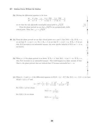
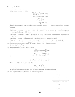
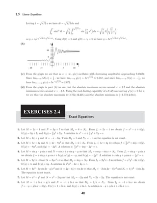
43. Separating variables we have dy/ 1 + y2 sin2
y = dx which
is not readily integrated (even by a CAS). We note that
dy/dx ≥ 0 for all values of x and y and that dy/dx = 0
when y = 0 and y = π, which are equilibrium solutions.
44. Separating variables we have dy/(
√
y + y) = dx/(
√
x + x). To integrate dx/(
√
x + x) we substitute u2
= x
and get
2u
u + u2
du =
2
1 + u
du = 2 ln |1 + u| + c = 2 ln(1 +
√
x ) + c.
Integrating the separated differential equation we have
2 ln(1 +
√
y ) = 2 ln(1 +
√
x ) + c or ln(1 +
√
y ) = ln(1 +
√
x ) + ln c1.
Solving for y we get y = [c1(1 +
√
x ) − 1]2
.
45. We are looking for a function y(x) such that
y2
+
dy
dx
2
= 1.
Using the positive square root gives
dy
dx
= 1 − y2 =⇒
dy
1 − y2
= dx =⇒ sin−1
y = x + c.
Thus a solution is y = sin(x + c). If we use the negative square root we obtain
y = sin(c − x) = − sin(x − c) = − sin(x + c1).
Note that when c = c1 = 0 and when c = c1 = π/2 we obtain the well known particular solutions y = sin x,
y = − sin x, y = cos x, and y = − cos x. Note also that y = 1 and y = −1 are singular solutions.
46. (a)
(b) For |x| > 1 and |y| > 1 the differential equation is dy/dx = y2 − 1 /
√
x2 − 1 . Separating variables and
integrating, we obtain
dy
y2 − 1
=
dx
√
x2 − 1
and cosh−1
y = cosh−1
x + c.
Setting x = 2 and y = 2 we find c = cosh−1
2 − cosh−1
2 = 0 and cosh−1
y = cosh−1
x. An explicit solution
is y = x.
47. Since the tension T1 (or magnitude T1) acts at the lowest point of the cable, we use symmetry to solve the
problem on the interval [0, L/2]. The assumption that the roadbed is uniform (that is, weighs a constant ρ
38

18. -4 -2 0 2 4
-4
-2
0
2
4
x
y
-4 -2 0 2 4
-4
-2
0
2
4
x
y
2.2 Separable Variables
pounds per horizontal foot) implies W = ρx, where x is measured in feet and 0 ≤ x ≤ L/2. Therefore (10)
becomes dy/dx = (ρ/T1)x. This last equation is a separable equation of the form given in (1) of Section 2.2 in
the text. Integrating and using the initial condition y(0) = a shows that the shape of the cable is a parabola:
y(x) = (ρ/2T1)x2
+a. In terms of the sag h of the cable and the span L, we see from Figure 2.22 in the text that
y(L/2) = h+a. By applying this last condition to y(x) = (ρ/2T1)x2
+a enables us to express ρ/2T1 in terms of
h and L: y(x) = (4h/L2
)x2
+ a. Since y(x) is an even function of x, the solution is valid on −L/2 ≤ x ≤ L/2.
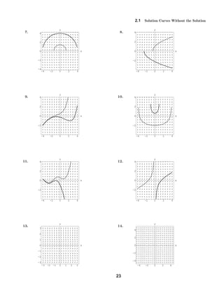
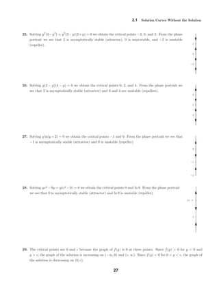
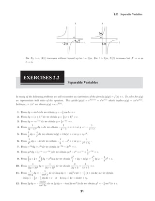
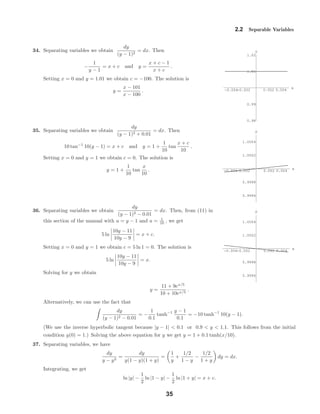
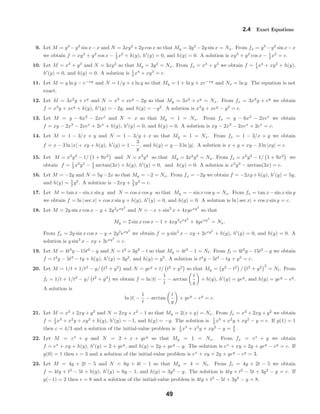
48. (a) Separating variables and integrating, we have (3y2
+1)dy = −(8x+5)dx
and y3
+ y = −4x2
− 5x + c. Using a CAS we show various contours
of f(x, y) = y3
+ y + 4x2
+ 5x. The plots shown on [−5, 5] × [−5, 5]
correspond to c-values of 0, ±5, ±20, ±40, ±80, and ±125.
(b) The value of c corresponding to y(0) = −1 is f(0, −1) = −2; to y(0) = 2 is
f(0, 2) = 10; to y(−1) = 4 is f(−1, 4) = 67; and to y(−1) = −3 is −31.
49. (a) An implicit solution of the differential equation (2y + 2)dy − (4x3
+ 6x)dx = 0 is
y2
+ 2y − x4
− 3x2
+ c = 0.
The condition y(0) = −3 implies that c = −3. Therefore y2
+ 2y − x4
− 3x2
− 3 = 0.
(b) Using the quadratic formula we can solve for y in terms of x:
y =
−2 ± 4 + 4(x4 + 3x2 + 3)
2
.
The explicit solution that satisfies the initial condition is then
y = −1 − x4 + 3x3 + 4 .
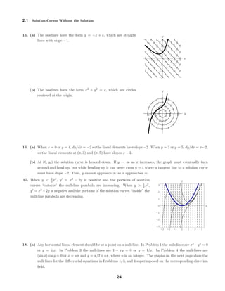
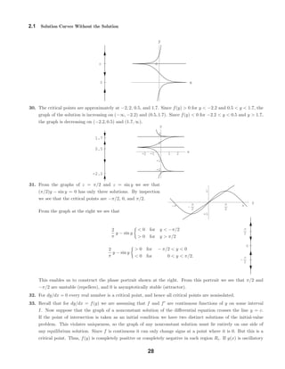
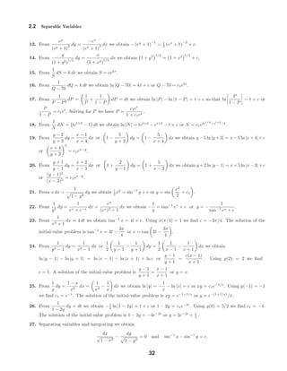
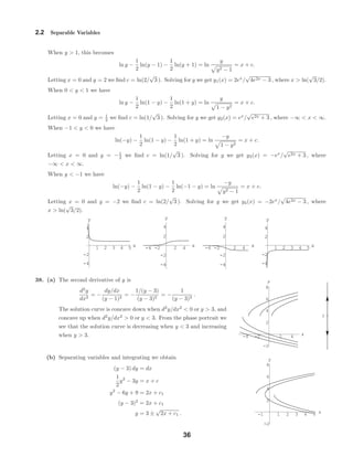
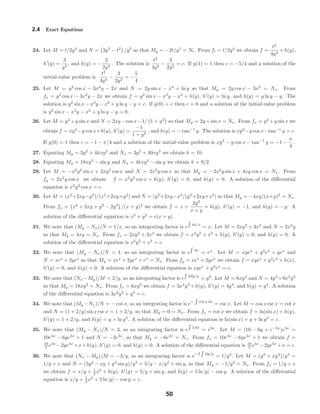
(c) From the graph of the function f(x) = x4
+3x3
+4 below we see that f(x) ≤ 0 on the approximate interval
−2.8 ≤ x ≤ −1.3. Thus the approximate domain of the function
y = −1 − x4 + 3x3 + 4 = −1 − f(x)
is x ≤ −2.8 or x ≥ −1.3. The graph of this function is shown below.
39

19. -4 -2 x
-4
-2
2
4
f x
-4 -2 2 x
-10
-8
-6
-4
-2
1 f x
2 x
-10
-8
-6
-4
-2
1 f x
-6 -4 -2 0 2 4 6
-4
-2
0
2
4
x
y
-2 0 2 4 6
-4
-2
0
2
4
x
y
2.2 Separable Variables
(d) Using the root finding capabilities of a CAS, the zeros of f are found to be −2.82202
and −1.3409. The domain of definition of the solution y(x) is then x > −1.3409. The
equality has been removed since the derivative dy/dx does not exist at the points where
f(x) = 0. The graph of the solution y = φ(x) is given on the right.
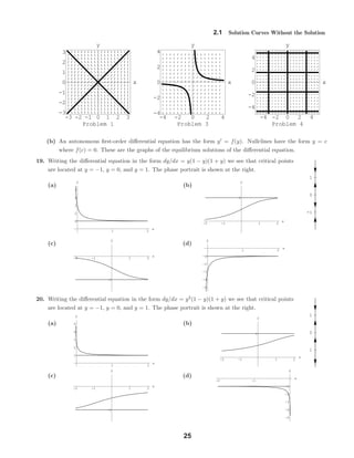
50. (a) Separating variables and integrating, we have
(−2y + y2
)dy = (x − x2
)dx
and
−y2
+
1
3
y3
=
1
2
x2
−
1
3
x3
+ c.
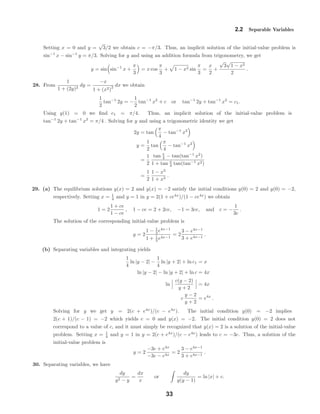
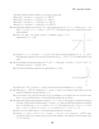
Using a CAS we show some contours of
f(x, y) = 2y3
− 6y2
+ 2x3
− 3x2
.
The plots shown on [−7, 7]×[−5, 5] correspond to c-values
of −450, −300, −200, −120, −60, −20, −10, −8.1, −5,
−0.8, 20, 60, and 120.
(b) The value of c corresponding to y(0) = 3
2 is f 0, 3
2 = −27
4 .
The portion of the graph between the dots corresponds to the
solution curve satisfying the intial condition. To determine the
interval of definition we find dy/dx for
2y3
− 6y2
+ 2x3
− 3x2
= −
27
4
.
Using implicit differentiation we get y = (x − x2
)/(y2
− 2y),
which is infinite when y = 0 and y = 2. Letting y = 0 in
2y3
− 6y2
+ 2x3
− 3x2
= −27
4 and using a CAS to solve for x
we get x = −1.13232. Similarly, letting y = 2, we find x = 1.71299. The largest interval of definition is
approximately (−1.13232, 1.71299).
40

20. -4 -2 0 2 4 6 8 10
-8
-6
-4
-2
0
2
4
x
y
2.3 Linear Equations
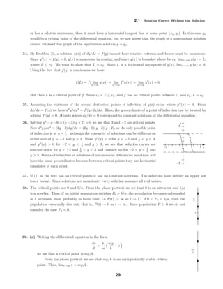
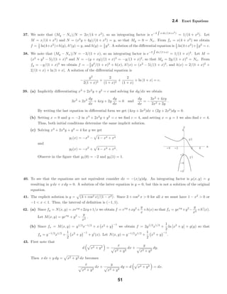
(c) The value of c corresponding to y(0) = −2 is f(0, −2) = −40.
The portion of the graph to the right of the dot corresponds to
the solution curve satisfying the initial condition. To determine
the interval of definition we find dy/dx for
2y3
− 6y2
+ 2x3
− 3x2
= −40.
Using implicit differentiation we get y = (x − x2
)/(y2
− 2y),
which is infinite when y = 0 and y = 2. Letting y = 0 in
2y3
− 6y2
+ 2x3
− 3x2
= −40 and using a CAS to solve for x
we get x = −2.29551. The largest interval of definition is approximately (−2.29551, ∞).
EXERCISES 2.3
Linear Equations
1. For y − 5y = 0 an integrating factor is e− 5 dx
= e−5x
so that
d
dx
e−5x
y = 0 and y = ce5x
for −∞ < x < ∞.
2. For y + 2y = 0 an integrating factor is e 2 dx
= e2x
so that
d
dx
e2x
y = 0 and y = ce−2x
for −∞ < x < ∞.
The transient term is ce−2x
.
3. For y +y = e3x
an integrating factor is e dx
= ex
so that
d
dx
[ex
y] = e4x
and y = 1
4 e3x
+ce−x
for −∞ < x < ∞.
The transient term is ce−x
.
4. For y + 4y = 4
3 an integrating factor is e 4 dx
= e4x
so that
d
dx
e4x
y = 4
3 e4x
and y = 1
3 + ce−4x
for
−∞ < x < ∞. The transient term is ce−4x
.
5. For y + 3x2
y = x2
an integrating factor is e 3x2
dx
= ex3
so that
d
dx
ex3
y = x2
ex3
and y = 1
3 + ce−x3
for
−∞ < x < ∞. The transient term is ce−x3
.
6. For y + 2xy = x3
an integrating factor is e 2x dx
= ex2
so that
d
dx
ex2
y = x3
ex2
and y = 1
2 x2
− 1
2 + ce−x2
for −∞ < x < ∞. The transient term is ce−x2
.
7. For y +
1
x
y =
1
x2
an integrating factor is e (1/x)dx
= x so that
d
dx
[xy] =
1
x
and y =
1
x
ln x+
c
x
for 0 < x < ∞.
8. For y − 2y = x2
+ 5 an integrating factor is e− 2 dx
= e−2x
so that
d
dx
e−2x
y = x2
e−2x
+ 5e−2x
and
y = −1
2 x2
− 1
2 x − 11
4 + ce2x
for −∞ < x < ∞.
9. For y −
1
x
y = x sin x an integrating factor is e− (1/x)dx
=
1
x
so that
d
dx
1
x
y = sin x and y = cx − x cos x for
0 < x < ∞.
10. For y +
2
x
y =
3
x
an integrating factor is e (2/x)dx
= x2
so that
d
dx
x2
y = 3x and y = 3
2 +cx−2
for 0 < x < ∞.
11. For y +
4
x
y = x2
−1 an integrating factor is e (4/x)dx
= x4
so that
d
dx
x4
y = x6
−x4
and y = 1
7 x3
− 1
5 x+cx−4
for 0 < x < ∞.
41

21. 2.3 Linear Equations
12. For y −
x
(1 + x)
y = x an integrating factor is e− [x/(1+x)]dx
= (x+1)e−x
so that
d
dx
(x + 1)e−x
y = x(x+1)e−x
and y = −x −
2x + 3
x + 1
+
cex
x + 1
for −1 < x < ∞.
13. For y + 1 +
2
x
y =
ex
x2
an integrating factor is e [1+(2/x)]dx
= x2
ex
so that
d
dx
[x2
ex
y] = e2x
and
y =
1
2
ex
x2
+
ce−x
x2
for 0 < x < ∞. The transient term is
ce−x
x2
.
14. For y + 1 +
1
x
y =
1
x
e−x
sin 2x an integrating factor is e [1+(1/x)]dx
= xex
so that
d
dx
[xex
y] = sin 2x and
y = −
1
2x
e−x
cos 2x +
ce−x
x
for 0 < x < ∞. The entire solution is transient.
15. For
dx
dy
−
4
y
x = 4y5
an integrating factor is e− (4/y)dy
= eln y−4
= y−4
so that
d
dy
y−4
x = 4y and x = 2y6
+cy4
for 0 < y < ∞.
16. For
dx
dy
+
2
y
x = ey
an integrating factor is e (2/y)dy
= y2
so that
d
dy
y2
x = y2
ey
and x = ey
−
2
y
ey
+
2
y2
ey
+
c
y2
for 0 < y < ∞. The transient term is
c
y2
.
17. For y + (tan x)y = sec x an integrating factor is e tan x dx
= sec x so that
d
dx
[(sec x)y] = sec2
x and
y = sin x + c cos x for −π/2 < x < π/2.
18. For y +(cot x)y = sec2
x csc x an integrating factor is e cot x dx
= eln | sin x|
= sin x so that
d
dx
[(sin x) y] = sec2
x
and y = sec x + c csc x for 0 < x < π/2.
19. For y +
x + 2
x + 1
y =
2xe−x
x + 1
an integrating factor is e [(x+2)/(x+1)]dx
= (x + 1)ex
, so
d
dx
[(x + 1)ex
y] = 2x and
y =
x2
x + 1
e−x
+
c
x + 1
e−x
for −1 < x < ∞. The entire solution is transient.
20. For y +
4
x + 2
y =
5
(x + 2)2
an integrating factor is e [4/(x+2)]dx
= (x + 2)4
so that
d
dx
(x + 2)4
y = 5(x + 2)2
and y =
5
3
(x + 2)−1
+ c(x + 2)−4
for −2 < x < ∞. The entire solution is transient.
21. For
dr
dθ
+ r sec θ = cos θ an integrating factor is e sec θ dθ
= eln | sec x+tan x|
= sec θ + tan θ so that
d
dθ
[(sec θ + tan θ)r] = 1 + sin θ and (sec θ + tan θ)r = θ − cos θ + c for −π/2 < θ < π/2 .
22. For
dP
dt
+ (2t − 1)P = 4t − 2 an integrating factor is e (2t−1) dt
= et2
−t
so that
d
dt
et2
−t
P = (4t − 2)et2
−t
and
P = 2 + cet−t2
for −∞ < t < ∞. The transient term is cet−t2
.
23. For y + 3 +
1
x
y =
e−3x
x
an integrating factor is e [3+(1/x)]dx
= xe3x
so that
d
dx
xe3x
y = 1 and
y = e−3x
+
ce−3x
x
for 0 < x < ∞. The transient term is ce−3x
/x.
24. For y +
2
x2 − 1
y =
x + 1
x − 1
an integrating factor is e [2/(x2
−1)]dx
=
x − 1
x + 1
so that
d
dx
x − 1
x + 1
y = 1 and
(x − 1)y = x(x + 1) + c(x + 1) for −1 < x < 1.
42

22. x
y
5
1
x
y
5
1
-1
x
y
3
2
2.3 Linear Equations
25. For y +
1
x
y =
1
x
ex
an integrating factor is e (1/x)dx
= x so that
d
dx
[xy] = ex
and y =
1
x
ex
+
c
x
for 0 < x < ∞.
If y(1) = 2 then c = 2 − e and y =
1
x
ex
+
2 − e
x
.
26. For
dx
dy
−
1
y
x = 2y an integrating factor is e− (1/y)dy
=
1
y
so that
d
dy
1
y
x = 2 and x = 2y2
+cy for 0 < y < ∞.
If y(1) = 5 then c = −49/5 and x = 2y2
−
49
5
y.
27. For
di
dt
+
R
L
i =
E
L
an integrating factor is e (R/L) dt
= eRt/L
so that
d
dt
eRt/L
i =
E
L
eRt/L
and
i =
E
R
+ ce−Rt/L
for −∞ < t < ∞. If i(0) = i0 then c = i0 − E/R and i =
E
R
+ i0 −
E
R
e−Rt/L
.
28. For
dT
dt
−kT = −Tmk an integrating factor is e (−k)dt
= e−kt
so that
d
dt
[e−kt
T] = −Tmke−kt
and T = Tm +cekt
for −∞ < t < ∞. If T(0) = T0 then c = T0 − Tm and T = Tm + (T0 − Tm)ekt
.
29. For y +
1
x + 1
y =
ln x
x + 1
an integrating factor is e [1/(x+1)]dx
= x + 1 so that
d
dx
[(x + 1)y] = ln x and
y =
x
x + 1
ln x −
x
x + 1
+
c
x + 1
for 0 < x < ∞. If y(1) = 10 then c = 21 and y =
x
x + 1
ln x −
x
x + 1
+
21
x + 1
.
30. For y + (tan x)y = cos2
x an integrating factor is e tan x dx
= eln | sec x|
= sec x so that
d
dx
[(sec x) y] = cos x
and y = sin x cos x + c cos x for −π/2 < x < π/2. If y(0) = −1 then c = −1 and y = sin x cos x − cos x.
31. For y + 2y = f(x) an integrating factor is e2x
so that
ye2x
=
1
2 e2x
+ c1, 0 ≤ x ≤ 3
c2, x > 3.
If y(0) = 0 then c1 = −1/2 and for continuity we must have c2 = 1
2 e6
− 1
2
so that
y =
1
2 (1 − e−2x
), 0 ≤ x ≤ 3
1
2 (e6
− 1)e−2x
, x > 3.
32. For y + y = f(x) an integrating factor is ex
so that
yex
=
ex
+ c1, 0 ≤ x ≤ 1
−ex
+ c2, x > 1.
If y(0) = 1 then c1 = 0 and for continuity we must have c2 = 2e so that
y =
1, 0 ≤ x ≤ 1
2e1−x
− 1, x > 1.
33. For y + 2xy = f(x) an integrating factor is ex2
so that
yex2
=
1
2 ex2
+ c1, 0 ≤ x ≤ 1
c2, x > 1.
If y(0) = 2 then c1 = 3/2 and for continuity we must have c2 = 1
2 e + 3
2
so that
y =
1
2 + 3
2 e−x2
, 0 ≤ x ≤ 1
1
2 e + 3
2 e−x2
, x > 1.
43

23. x
y
5
-1
1
x
y
3
5
10
15
20
2.3 Linear Equations
34. For
y +
2x
1 + x2
y =



x
1 + x2
, 0 ≤ x ≤ 1
−x
1 + x2
, x > 1,
an integrating factor is 1 + x2
so that
1 + x2
y =
1
2 x2
+ c1, 0 ≤ x ≤ 1
−1
2 x2
+ c2, x > 1.
If y(0) = 0 then c1 = 0 and for continuity we must have c2 = 1 so that
y =



1
2
−
1
2 (1 + x2)
, 0 ≤ x ≤ 1
3
2 (1 + x2)
−
1
2
, x > 1.
35. We first solve the initial-value problem y + 2y = 4x, y(0) = 3 on the interval [0, 1].
The integrating factor is e 2 dx
= e2x
, so
d
dx
[e2x
y] = 4xe2x
e2x
y = 4xe2x
dx = 2xe2x
− e2x
+ c1
y = 2x − 1 + c1e−2x
.
Using the initial condition, we find y(0) = −1+c1 = 3, so c1 = 4 and y = 2x−1+4e−2x
,
0 ≤ x ≤ 1. Now, since y(1) = 2−1+4e−2
= 1+4e−2
, we solve the initial-value problem
y − (2/x)y = 4x, y(1) = 1 + 4e−2
on the interval (1, ∞). The integrating factor is
e (−2/x)dx
= e−2 ln x
= x−2
, so
d
dx
[x−2
y] = 4xx−2
=
4
x
x−2
y =
4
x
dx = 4 ln x + c2
y = 4x2
ln x + c2x2
.
(We use ln x instead of ln |x| because x > 1.) Using the initial condition we find y(1) = c2 = 1 + 4e−2
, so
y = 4x2
ln x + (1 + 4e−2
)x2
, x > 1. Thus, the solution of the original initial-value problem is
y =
2x − 1 + 4e−2x
, 0 ≤ x ≤ 1
4x2
ln x + (1 + 4e−2
)x2
, x > 1.
See Problem 42 in this section.
36. For y + ex
y = 1 an integrating factor is eex
. Thus
d
dx
eex
y = eex
and eex
y =
x
0
eet
dt + c.
From y(0) = 1 we get c = e, so y = e−ex x
0
eet
dt + e1−ex
.
When y + ex
y = 0 we can separate variables and integrate:
dy
y
= −ex
dx and ln |y| = −ex
+ c.
44

24. 2.3 Linear Equations
Thus y = c1e−ex
. From y(0) = 1 we get c1 = e, so y = e1−ex
.
When y + ex
y = ex
we can see by inspection that y = 1 is a solution.
37. An integrating factor for y − 2xy = 1 is e−x2
. Thus
d
dx
[e−x2
y] = e−x2
e−x2
y =
x
0
e−t2
dt =
√
π
2
erf(x) + c
y =
√
π
2
ex2
erf(x) + cex2
.
From y(1) = (
√
π/2)e erf(1) + ce = 1 we get c = e−1
−
√
π
2 erf(1). The solution of the initial-value problem is
y =
√
π
2
ex2
erf(x) + e−1
−
√
π
2
erf(1) ex2
= ex2
−1
+
√
π
2
ex2
(erf(x) − erf(1)).
38. We want 4 to be a critical point, so we use y = 4 − y.
39. (a) All solutions of the form y = x5
ex
− x4
ex
+ cx4
satisfy the initial condition. In this case, since 4/x is
discontinuous at x = 0, the hypotheses of Theorem 1.1 are not satisfied and the initial-value problem does
not have a unique solution.
(b) The differential equation has no solution satisfying y(0) = y0, y0 > 0.
(c) In this case, since x0 > 0, Theorem 1.1 applies and the initial-value problem has a unique solution given by
y = x5
ex
− x4
ex
+ cx4
where c = y0/x4
0 − x0ex0
+ ex0
.
40. On the interval (−3, 3) the integrating factor is
e x dx/(x2
−9)
= e− x dx/(9−x2
)
= e
1
2 ln(9−x2
)
= 9 − x2
and so
d
dx
9 − x2 y = 0 and y =
c
√
9 − x2
.
41. We want the general solution to be y = 3x − 5 + ce−x
. (Rather than e−x
, any function that approaches 0 as
x → ∞ could be used.) Differentiating we get
y = 3 − ce−x
= 3 − (y − 3x + 5) = −y + 3x − 2,
so the differential equation y + y = 3x − 2 has solutions asymptotic to the line y = 3x − 5.
42. The left-hand derivative of the function at x = 1 is 1/e and the right-hand derivative at x = 1 is 1 − 1/e. Thus,
y is not differentiable at x = 1.
43. (a) Differentiating yc = c/x3
we get
yc = −
3c
x4
= −
3
x
c
x3
= −
3
x
yc
so a differential equation with general solution yc = c/x3
is xy + 3y = 0. Now
xyp + 3yp = x(3x2
) + 3(x3
) = 6x3
so a differential equation with general solution y = c/x3
+ x3
is xy + 3y = 6x3
. This will be a general
solution on (0, ∞).
45

25. x
y
5
-3
3
2.3 Linear Equations
(b) Since y(1) = 13
− 1/13
= 0, an initial condition is y(1) = 0. Since
y(1) = 13
+ 2/13
= 3, an initial condition is y(1) = 3. In each case the
interval of definition is (0, ∞). The initial-value problem xy + 3y = 6x3
,
y(0) = 0 has solution y = x3
for −∞ < x < ∞. In the figure the lower
curve is the graph of y(x) = x3
−1/x3
,while the upper curve is the graph
of y = x3
− 2/x3
.
(c) The first two initial-value problems in part (b) are not unique. For example, setting
y(2) = 23
− 1/23
= 63/8, we see that y(2) = 63/8 is also an initial condition leading to the solution
y = x3
− 1/x3
.
44. Since e P (x)dx+c
= ec
e P (x)dx
= c1e P (x)dx
, we would have
c1e P (x)dx
y = c2 + c1e P (x)dx
f(x) dx and e P (x)dx
y = c3 + e P (x)dx
f(x) dx,
which is the same as (6) in the text.
45. We see by inspection that y = 0 is a solution.
46. The solution of the first equation is x = c1e−λ1t
. From x(0) = x0 we obtain c1 = x0 and so x = x0e−λ1t
. The
second equation then becomes
dy
dt
= x0λ1e−λ1t
− λ2y or
dy
dt
+ λ2y = x0λ1e−λ1t
which is linear. An integrating factor is eλ2t
. Thus
d
dt
[eλ2t
y ] = x0λ1e−λ1t
eλ2t
= x0λ1e(λ2−λ1)t
eλ2t
y =
x0λ1
λ2 − λ1
e(λ2−λ1)t
+ c2
y =
x0λ1
λ2 − λ1
e−λ1t
+ c2e−λ2t
.
From y(0) = y0 we obtain c2 = (y0λ2 − y0λ1 − x0λ1)/(λ2 − λ1). The solution is
y =
x0λ1
λ2 − λ1
e−λ1t
+
y0λ2 − y0λ1 − x0λ1
λ2 − λ1
e−λ2t
.
47. Writing the differential equation as
dE
dt
+
1
RC
E = 0 we see that an integrating factor is et/RC
. Then
d
dt
[et/RC
E] = 0
et/RC
E = c
E = ce−t/RC
.
From E(4) = ce−4/RC
= E0 we find c = E0e4/RC
. Thus, the solution of the initial-value problem is
E = E0e4/RC
e−t/RC
= E0e−(t−4)/RC
.
46

26. x
y
5
5
1 2 3 4 5
x
-5
-4
-3
-2
-1
1
2
y
2.3 Linear Equations
48. (a) An integrating factor for y − 2xy = −1 is e−x2
. Thus
d
dx
[e−x2
y] = −e−x2
e−x2
y = −
x
0
e−t2
dt = −
√
π
2
erf(x) + c.
From y(0) =
√
π/2, and noting that erf(0) = 0, we get c =
√
π/2. Thus
y = ex2
−
√
π
2
erf(x) +
√
π
2
=
√
π
2
ex2
(1 − erf(x)) =
√
π
2
ex2
erfc(x).
(b) Using a CAS we find y(2) ≈ 0.226339.
49. (a) An integrating factor for
y +
2
x
y =
10 sin x
x3
is x2
. Thus
d
dx
[x2
y] = 10
sin x
x
x2
y = 10
x
0
sin t
t
dt + c
y = 10x−2
Si(x) + cx−2
.
From y(1) = 0 we get c = −10Si(1). Thus
y = 10x−2
Si(x) − 10x−2
Si(1) = 10x−2
(Si(x) − Si(1)).
(b)
(c) From the graph in part (b) we see that the absolute maximum occurs around x = 1.7. Using the root-finding
capability of a CAS and solving y (x) = 0 for x we see that the absolute maximum is (1.688, 1.742).
50. (a) The integrating factor for y − (sin x2
)y = 0 is e
−
x
0
sin t2
dt
. Then
d
dx
[e
−
x
0
sin t2
dt
y] = 0
e
−
x
0
sin t2
dt
y = c1
y = c1e
x
0
sin t2
dt
.
47

27. x
y
-10 -5 5 10
5
10
2.3 Linear Equations
Letting t = π/2 u we have dt = π/2 du and
x
0
sin t2
dt =
π
2
√
2/π x
0
sin
π
2
u2
du =
π
2
S
2
π
x
so y = c1e
√
π/2 S(
√
2/π x)
. Using S(0) = 0 and y(0) = c1 = 5 we have y = 5e
√
π/2 S(
√
2/π x)
.
(b)
(c) From the graph we see that as x → ∞, y(x) oscillates with decreasing amplitudes approaching 9.35672.
Since limx→∞ 5S(x) = 1
2 , we have limx→∞ y(x) = 5e
√
π/8
≈ 9.357, and since limx→−∞ S(x) = −1
2 , we
have limx→−∞ y(x) = 5e−
√
π/8
≈ 2.672.
(d) From the graph in part (b) we see that the absolute maximum occurs around x = 1.7 and the absolute
minimum occurs around x = −1.8. Using the root-finding capability of a CAS and solving y (x) = 0 for x,
we see that the absolute maximum is (1.772, 12.235) and the absolute minimum is (−1.772, 2.044).
EXERCISES 2.4
Exact Equations
1. Let M = 2x − 1 and N = 3y + 7 so that My = 0 = Nx. From fx = 2x − 1 we obtain f = x2
− x + h(y),
h (y) = 3y + 7, and h(y) = 3
2 y2
+ 7y. A solution is x2
− x + 3
2 y2
+ 7y = c.
2. Let M = 2x + y and N = −x − 6y. Then My = 1 and Nx = −1, so the equation is not exact.
3. Let M = 5x + 4y and N = 4x − 8y3
so that My = 4 = Nx. From fx = 5x + 4y we obtain f = 5
2 x2
+ 4xy + h(y),
h (y) = −8y3
, and h(y) = −2y4
. A solution is 5
2 x2
+ 4xy − 2y4
= c.
4. Let M = sin y − y sin x and N = cos x + x cos y − y so that My = cos y − sin x = Nx. From fx = sin y − y sin x
we obtain f = x sin y + y cos x + h(y), h (y) = −y, and h(y) = −1
2 y2
. A solution is x sin y + y cos x − 1
2 y2
= c.
5. Let M = 2y2
x−3 and N = 2yx2
+4 so that My = 4xy = Nx. From fx = 2y2
x−3 we obtain f = x2
y2
−3x+h(y),
h (y) = 4, and h(y) = 4y. A solution is x2
y2
− 3x + 4y = c.
6. Let M = 4x3
−3y sin 3x−y/x2
and N = 2y−1/x+cos 3x so that My = −3 sin 3x−1/x2
and Nx = 1/x2
−3 sin 3x.
The equation is not exact.
7. Let M = x2
− y2
and N = x2
− 2xy so that My = −2y and Nx = 2x − 2y. The equation is not exact.
8. Let M = 1 + ln x + y/x and N = −1 + ln x so that My = 1/x = Nx. From fy = −1 + ln x we obtain
f = −y + y ln x + h(y), h (x) = 1 + ln x, and h(y) = x ln x. A solution is −y + y ln x + x ln x = c.
48

28. 2.4 Exact Equations
9. Let M = y3
−y2
sin x−x and N = 3xy2
+2y cos x so that My = 3y2
−2y sin x = Nx. From fx = y3
−y2
sin x−x
we obtain f = xy3
+ y2
cos x − 1
2 x2
+ h(y), h (y) = 0, and h(y) = 0. A solution is xy3
+ y2
cos x − 1
2 x2
= c.
10. Let M = x3
+ y3
and N = 3xy2
so that My = 3y2
= Nx. From fx = x3
+ y3
we obtain f = 1
4 x4
+ xy3
+ h(y),
h (y) = 0, and h(y) = 0. A solution is 1
4 x4
+ xy3
= c.
11. Let M = y ln y − e−xy
and N = 1/y + x ln y so that My = 1 + ln y + xe−xy
and Nx = ln y. The equation is not
exact.
12. Let M = 3x2
y + ey
and N = x3
+ xey
− 2y so that My = 3x2
+ ey
= Nx. From fx = 3x2
y + ey
we obtain
f = x3
y + xey
+ h(y), h (y) = −2y, and h(y) = −y2
. A solution is x3
y + xey
− y2
= c.
13. Let M = y − 6x2
− 2xex
and N = x so that My = 1 = Nx. From fx = y − 6x2
− 2xex
we obtain
f = xy − 2x3
− 2xex
+ 2ex
+ h(y), h (y) = 0, and h(y) = 0. A solution is xy − 2x3
− 2xex
+ 2ex
= c.
14. Let M = 1 − 3/x + y and N = 1 − 3/y + x so that My = 1 = Nx. From fx = 1 − 3/x + y we obtain
f = x − 3 ln |x| + xy + h(y), h (y) = 1 −
3
y
, and h(y) = y − 3 ln |y|. A solution is x + y + xy − 3 ln |xy| = c.
15. Let M = x2
y3
− 1/ 1 + 9x2
and N = x3
y2
so that My = 3x2
y2
= Nx. From fx = x2
y3
− 1/ 1 + 9x2
we
obtain f = 1
3 x3
y3
− 1
3 arctan(3x) + h(y), h (y) = 0, and h(y) = 0. A solution is x3
y3
− arctan(3x) = c.
16. Let M = −2y and N = 5y−2x so that My = −2 = Nx. From fx = −2y we obtain f = −2xy+h(y), h (y) = 5y,
and h(y) = 5
2 y2
. A solution is −2xy + 5
2 y2
= c.
17. Let M = tan x−sin x sin y and N = cos x cos y so that My = − sin x cos y = Nx. From fx = tan x−sin x sin y
we obtain f = ln | sec x| + cos x sin y + h(y), h (y) = 0, and h(y) = 0. A solution is ln | sec x| + cos x sin y = c.
18. Let M = 2y sin x cos x − y + 2y2
exy2
and N = −x + sin2
x + 4xyexy2
so that
My = 2 sin x cos x − 1 + 4xy3
exy2
+ 4yexy2
= Nx.
From fx = 2y sin x cos x − y + 2y2
exy2
we obtain f = y sin2
x − xy + 2exy2
+ h(y), h (y) = 0, and h(y) = 0. A
solution is y sin2
x − xy + 2exy2
= c.
19. Let M = 4t3
y − 15t2
− y and N = t4
+ 3y2
− t so that My = 4t3
− 1 = Nt. From ft = 4t3
y − 15t2
− y we obtain
f = t4
y − 5t3
− ty + h(y), h (y) = 3y2
, and h(y) = y3
. A solution is t4
y − 5t3
− ty + y3
= c.
20. Let M = 1/t + 1/t2
− y/ t2
+ y2
and N = yey
+ t/ t2
+ y2
so that My = y2
− t2
/ t2
+ y2 2
= Nt. From
ft = 1/t + 1/t2
− y/ t2
+ y2
we obtain f = ln |t| −
1
t
− arctan
t
y
+ h(y), h (y) = yey
, and h(y) = yey
− ey
.
A solution is
ln |t| −
1
t
− arctan
t
y
+ yey
− ey
= c.
21. Let M = x2
+ 2xy + y2
and N = 2xy + x2
− 1 so that My = 2(x + y) = Nx. From fx = x2
+ 2xy + y2
we obtain
f = 1
3 x3
+ x2
y + xy2
+ h(y), h (y) = −1, and h(y) = −y. The solution is 1
3 x3
+ x2
y + xy2
− y = c. If y(1) = 1
then c = 4/3 and a solution of the initial-value problem is 1
3 x3
+ x2
y + xy2
− y = 4
3 .
22. Let M = ex
+ y and N = 2 + x + yey
so that My = 1 = Nx. From fx = ex
+ y we obtain
f = ex
+ xy + h(y), h (y) = 2 + yey
, and h(y) = 2y + yey
− y. The solution is ex
+ xy + 2y + yey
− ey
= c. If
y(0) = 1 then c = 3 and a solution of the initial-value problem is ex
+ xy + 2y + yey
− ey
= 3.
23. Let M = 4y + 2t − 5 and N = 6y + 4t − 1 so that My = 4 = Nt. From ft = 4y + 2t − 5 we obtain
f = 4ty + t2
− 5t + h(y), h (y) = 6y − 1, and h(y) = 3y2
− y. The solution is 4ty + t2
− 5t + 3y2
− y = c. If
y(−1) = 2 then c = 8 and a solution of the initial-value problem is 4ty + t2
− 5t + 3y2
− y = 8.
49

29. 2.4 Exact Equations
24. Let M = t/2y4
and N = 3y2
− t2
/y5
so that My = −2t/y5
= Nt. From ft = t/2y4
we obtain f =
t2
4y4
+h(y),
h (y) =
3
y3
, and h(y) = −
3
2y2
. The solution is
t2
4y4
−
3
2y2
= c. If y(1) = 1 then c = −5/4 and a solution of the
initial-value problem is
t2
4y4
−
3
2y2
= −
5
4
.
25. Let M = y2
cos x − 3x2
y − 2x and N = 2y sin x − x3
+ ln y so that My = 2y cos x − 3x2
= Nx. From
fx = y2
cos x − 3x2
y − 2x we obtain f = y2
sin x − x3
y − x2
+ h(y), h (y) = ln y, and h(y) = y ln y − y. The
solution is y2
sin x − x3
y − x2
+ y ln y − y = c. If y(0) = e then c = 0 and a solution of the initial-value problem
is y2
sin x − x3
y − x2
+ y ln y − y = 0.
26. Let M = y2
+y sin x and N = 2xy −cos x−1/ 1 + y2
so that My = 2y +sin x = Nx. From fx = y2
+y sin x we
obtain f = xy2
−y cos x+h(y), h (y) =
−1
1 + y2
, and h(y) = − tan−1
y. The solution is xy2
−y cos x−tan−1
y = c.
If y(0) = 1 then c = −1 − π/4 and a solution of the initial-value problem is xy2
− y cos x − tan−1
y = −1 −
π
4
.
27. Equating My = 3y2
+ 4kxy3
and Nx = 3y2
+ 40xy3
we obtain k = 10.
28. Equating My = 18xy2
− sin y and Nx = 4kxy2
− sin y we obtain k = 9/2.
29. Let M = −x2
y2
sin x + 2xy2
cos x and N = 2x2
y cos x so that My = −2x2
y sin x + 4xy cos x = Nx. From
fy = 2x2
y cos x we obtain f = x2
y2
cos x + h(y), h (y) = 0, and h(y) = 0. A solution of the differential
equation is x2
y2
cos x = c.
30. Let M = (x2
+2xy−y2
)/(x2
+2xy+y2
) and N = (y2
+2xy−x2
/(y2
+2xy+x2
) so that My = −4xy/(x+y)3
= Nx.
From fx = x2
+ 2xy + y2
− 2y2
/(x + y)2
we obtain f = x +
2y2
x + y
+ h(y), h (y) = −1, and h(y) = −y. A
solution of the differential equation is x2
+ y2
= c(x + y).
31. We note that (My − Nx)/N = 1/x, so an integrating factor is e dx/x
= x. Let M = 2xy2
+ 3x2
and N = 2x2
y
so that My = 4xy = Nx. From fx = 2xy2
+ 3x2
we obtain f = x2
y2
+ x3
+ h(y), h (y) = 0, and h(y) = 0. A
solution of the differential equation is x2
y2
+ x3
= c.
32. We note that (My − Nx)/N = 1, so an integrating factor is e dx
= ex
. Let M = xyex
+ y2
ex
+ yex
and
N = xex
+ 2yex
so that My = xex
+ 2yex
+ ex
= Nx. From fy = xex
+ 2yex
we obtain f = xyex
+ y2
ex
+ h(x),
h (y) = 0, and h(y) = 0. A solution of the differential equation is xyex
+ y2
ex
= c.
33. We note that (Nx −My)/M = 2/y, so an integrating factor is e 2dy/y
= y2
. Let M = 6xy3
and N = 4y3
+9x2
y2
so that My = 18xy2
= Nx. From fx = 6xy3
we obtain f = 3x2
y3
+h(y), h (y) = 4y3
, and h(y) = y4
. A solution
of the differential equation is 3x2
y3
+ y4
= c.
34. We note that (My −Nx)/N = − cot x, so an integrating factor is e− cot x dx
= csc x. Let M = cos x csc x = cot x
and N = (1 + 2/y) sin x csc x = 1 + 2/y, so that My = 0 = Nx. From fx = cot x we obtain f = ln(sin x) + h(y),
h (y) = 1 + 2/y, and h(y) = y + ln y2
. A solution of the differential equation is ln(sin x) + y + ln y2
= c.
35. We note that (My − Nx)/N = 3, so an integrating factor is e 3 dx
= e3x
. Let M = (10 − 6y + e−3x
)e3x
=
10e3x
− 6ye3x
+ 1 and N = −2e3x
, so that My = −6e3x
= Nx. From fx = 10e3x
− 6ye3x
+ 1 we obtain f =
10
3 e3x
−2ye3x
+x+h(y), h (y) = 0, and h(y) = 0. A solution of the differential equation is 10
3 e3x
−2ye3x
+x = c.
36. We note that (Nx − My)/M = −3/y, so an integrating factor is e−3 dy/y
= 1/y3
. Let M = (y2
+ xy3
)/y3
=
1/y + x and N = (5y2
− xy + y3
sin y)/y3
= 5/y − x/y2
+ sin y, so that My = −1/y2
= Nx. From fx = 1/y + x
we obtain f = x/y + 1
2 x2
+ h(y), h (y) = 5/y + sin y, and h(y) = 5 ln |y| − cos y. A solution of the differential
equation is x/y + 1
2 x2
+ 5 ln |y| − cos y = c.
50

30. -4 -2 2 4 x
-6
-4
-2
2
4
y
y1
y2
2.4 Exact Equations
37. We note that (My − Nx)/N = 2x/(4 + x2
), so an integrating factor is e−2 x dx/(4+x2
)
= 1/(4 + x2
). Let
M = x/(4 + x2
) and N = (x2
y + 4y)/(4 + x2
) = y, so that My = 0 = Nx. From fx = x(4 + x2
) we obtain
f = 1
2 ln(4+x2
)+h(y), h (y) = y, and h(y) = 1
2 y2
. A solution of the differential equation is 1
2 ln(4+x2
)+ 1
2 y2
= c.
38. We note that (My − Nx)/N = −3/(1 + x), so an integrating factor is e−3 dx/(1+x)
= 1/(1 + x)3
. Let M =
(x2
+ y2
− 5)/(1 + x)3
and N = −(y + xy)/(1 + x)3
= −y/(1 + x)2
, so that My = 2y/(1 + x)3
= Nx. From
fy = −y/(1 + x)2
we obtain f = −1
2 y2
/(1 + x)2
+ h(x), h (x) = (x2
− 5)/(1 + x)3
, and h(x) = 2/(1 + x)2
+
2/(1 + x) + ln |1 + x|. A solution of the differential equation is
−
y2
2(1 + x)2
+
2
(1 + x)2
+
2
(1 + x)
+ ln |1 + x| = c.
39. (a) Implicitly differentiating x3
+ 2x2
y + y2
= c and solving for dy/dx we obtain
3x2
+ 2x2 dy
dx
+ 4xy + 2y
dy
dx
= 0 and
dy
dx
= −
3x2
+ 4xy
2x2 + 2y
.
By writing the last equation in differential form we get (4xy + 3x2
)dx + (2y + 2x2
)dy = 0.
(b) Setting x = 0 and y = −2 in x3
+ 2x2
y + y2
= c we find c = 4, and setting x = y = 1 we also find c = 4.
Thus, both initial conditions determine the same implicit solution.
(c) Solving x3
+ 2x2
y + y2
= 4 for y we get
y1(x) = −x2
− 4 − x3 + x4
and
y2(x) = −x2
+ 4 − x3 + x4 .
Observe in the figure that y1(0) = −2 and y2(1) = 1.
40. To see that the equations are not equivalent consider dx = −(x/y)dy. An integrating factor is µ(x, y) = y
resulting in y dx + x dy = 0. A solution of the latter equation is y = 0, but this is not a solution of the original
equation.
41. The explicit solution is y = (3 + cos2 x)/(1 − x2) . Since 3 + cos2
x > 0 for all x we must have 1 − x2
> 0 or
−1 < x < 1. Thus, the interval of definition is (−1, 1).
42. (a) Since fy = N(x, y) = xexy
+2xy+1/x we obtain f = exy
+xy2
+
y
x
+h(x) so that fx = yexy
+y2
−
y
x2
+h (x).
Let M(x, y) = yexy
+ y2
−
y
x2
.
(b) Since fx = M(x, y) = y1/2
x−1/2
+ x x2
+ y
−1
we obtain f = 2y1/2
x1/2
+
1
2
ln x2
+ y + g(y) so that
fy = y−1/2
x1/2
+
1
2
x2
+ y
−1
+ g (x). Let N(x, y) = y−1/2
x1/2
+
1
2
x2
+ y
−1
.
43. First note that
d x2 + y2 =
x
x2 + y2
dx +
y
x2 + y2
dy.
Then x dx + y dy = x2 + y2 dx becomes
x
x2 + y2
dx +
y
x2 + y2
dy = d x2 + y2 = dx.
51

31. 2.4 Exact Equations
The left side is the total differential of x2 + y2 and the right side is the total differential of x + c. Thus
x2 + y2 = x + c is a solution of the differential equation.
44. To see that the statement is true, write the separable equation as −g(x) dx+dy/h(y) = 0. Identifying M = −g(x)
and N = 1/h(y), we see that My = 0 = Nx, so the differential equation is exact.
45. (a) In differential form we have (v2
− 32x)dx + xv dv = 0. This is not an exact form, but µ(x) = x is an
integrating factor. Multiplying by x we get (xv2
− 32x2
)dx + x2
v dv = 0. This form is the total differential
of u = 1
2 x2
v2
− 32
3 x3
, so an implicit solution is 1
2 x2
v2
− 32
3 x3
= c. Letting x = 3 and v = 0 we find c = −288.
Solving for v we get
v = 8
x
3
−
9
x2
.
(b) The chain leaves the platform when x = 8, so the velocity at this time is
v(8) = 8
8
3
−
9
64
≈ 12.7 ft/s.
46. (a) Letting
M(x, y) =
2xy
(x2 + y2)2
and N(x, y) = 1 +
y2
− x2
(x2 + y2)2
we compute
My =
2x3
− 8xy2
(x2 + y2)3
= Nx,
so the differential equation is exact. Then we have
∂f
∂x
= M(x, y) =
2xy
(x2 + y2)2
= 2xy(x2
+ y2
)−2
f(x, y) = −y(x2
+ y2
)−1
+ g(y) = −
y
x2 + y2
+ g(y)
∂f
∂y
=
y2
− x2
(x2 + y2)2
+ g (y) = N(x, y) = 1 +
y2
− x2
(x2 + y2)2
.
Thus, g (y) = 1 and g(y) = y. The solution is y −
y
x2 + y2
= c. When c = 0 the solution is x2
+ y2
= 1.
(b) The first graph below is obtained in Mathematica using f(x, y) = y − y/(x2
+ y2
) and
ContourPlot[f[x, y], {x, -3, 3}, {y, -3, 3},
Axes−>True, AxesOrigin−>{0, 0}, AxesLabel−>{x, y},
Frame−>False, PlotPoints−>100, ContourShading−>False,
Contours−>{0, -0.2, 0.2, -0.4, 0.4, -0.6, 0.6, -0.8, 0.8}]
The second graph uses
x = −
y3 − cy2 − y
c − y
and x =
y3 − cy2 − y
c − y
.
In this case the x-axis is vertical and the y-axis is horizontal. To obtain the third graph, we solve
y − y/(x2
+ y2
) = c for y in a CAS. This appears to give one real and two complex solutions. When
graphed in Mathematica however, all three solutions contribute to the graph. This is because the solutions
involve the square root of expressions containing c. For some values of c the expression is negative, causing
an apparent complex solution to actually be real.
52

32. -3 -2 -1 1 2 3
x
-3
-2
-1
1
2
3
y
-1.5-1-0.5 0.511.5y
-3
-2
-1
1
2
3
x
-3 -2 -1 1 2 3
-3
-2
-1
1
2
3
y
2.5 Solutions by Substitutions
EXERCISES 2.5
Solutions by Substitutions
1. Letting y = ux we have
(x − ux) dx + x(u dx + x du) = 0
dx + x du = 0
dx
x
+ du = 0
ln |x| + u = c
x ln |x| + y = cx.
2. Letting y = ux we have
(x + ux) dx + x(u dx + x du) = 0
(1 + 2u) dx + x du = 0
dx
x
+
du
1 + 2u
= 0
ln |x| +
1
2
ln |1 + 2u| = c
x2
1 + 2
y
x
= c1
x2
+ 2xy = c1.
53

33. 2.5 Solutions by Substitutions
3. Letting x = vy we have
vy(v dy + y dv) + (y − 2vy) dy = 0
vy2
dv + y v2
− 2v + 1 dy = 0
v dv
(v − 1)2
+
dy
y
= 0
ln |v − 1| −
1
v − 1
+ ln |y| = c
ln
x
y
− 1 −
1
x/y − 1
+ ln y = c
(x − y) ln |x − y| − y = c(x − y).
4. Letting x = vy we have
y(v dy + y dv) − 2(vy + y) dy = 0
y dv − (v + 2) dy = 0
dv
v + 2
−
dy
y
= 0
ln |v + 2| − ln |y| = c
ln
x
y
+ 2 − ln |y| = c
x + 2y = c1y2
.
5. Letting y = ux we have
u2
x2
+ ux2
dx − x2
(u dx + x du) = 0
u2
dx − x du = 0
dx
x
−
du
u2
= 0
ln |x| +
1
u
= c
ln |x| +
x
y
= c
y ln |x| + x = cy.
6. Letting y = ux and using partial fractions, we have
u2
x2
+ ux2
dx + x2
(u dx + x du) = 0
x2
u2
+ 2u dx + x3
du = 0
dx
x
+
du
u(u + 2)
= 0
ln |x| +
1
2
ln |u| −
1
2
ln |u + 2| = c
x2
u
u + 2
= c1
x2 y
x
= c1
y
x
+ 2
x2
y = c1(y + 2x).
54

34. 2.5 Solutions by Substitutions
7. Letting y = ux we have
(ux − x) dx − (ux + x)(u dx + x du) = 0
u2
+ 1 dx + x(u + 1) du = 0
dx
x
+
u + 1
u2 + 1
du = 0
ln |x| +
1
2
ln u2
+ 1 + tan−1
u = c
ln x2 y2
x2
+ 1 + 2 tan−1 y
x
= c1
ln x2
+ y2
+ 2 tan−1 y
x
= c1.
8. Letting y = ux we have
(x + 3ux) dx − (3x + ux)(u dx + x du) = 0
u2
− 1 dx + x(u + 3) du = 0
dx
x
+
u + 3
(u − 1)(u + 1)
du = 0
ln |x| + 2 ln |u − 1| − ln |u + 1| = c
x(u − 1)2
u + 1
= c1
x
y
x
− 1
2
= c1
y
x
+ 1
(y − x)2
= c1(y + x).
9. Letting y = ux we have
−ux dx + (x +
√
u x)(u dx + x du) = 0
(x2
+ x2
√
u ) du + xu3/2
dx = 0
u−3/2
+
1
u
du +
dx
x
= 0
−2u−1/2
+ ln |u| + ln |x| = c
ln |y/x| + ln |x| = 2 x/y + c
y(ln |y| − c)2
= 4x.
10. Letting y = ux we have
ux + x2 − (ux)2 dx − x(udx + xdu) du = 0
x2 − u2x2 dx − x2
du = 0
x 1 − u2 dx − x2
du = 0, (x > 0)
dx
x
−
du
√
1 − u2
= 0
ln x − sin−1
u = c
sin−1
u = ln x + c1
55

35. 2.5 Solutions by Substitutions
sin−1 y
x
= ln x + c2
y
x
= sin(ln x + c2)
y = x sin(ln x + c2).
See Problem 33 in this section for an analysis of the solution.
11. Letting y = ux we have
x3
− u3
x3
dx + u2
x3
(u dx + x du) = 0
dx + u2
x du = 0
dx
x
+ u2
du = 0
ln |x| +
1
3
u3
= c
3x3
ln |x| + y3
= c1x3
.
Using y(1) = 2 we find c1 = 8. The solution of the initial-value problem is 3x3
ln |x| + y3
= 8x3
.
12. Letting y = ux we have
(x2
+ 2u2
x2
)dx − ux2
(u dx + x du) = 0
x2
(1 + u2
)dx − ux3
du = 0
dx
x
−
u du
1 + u2
= 0
ln |x| −
1
2
ln(1 + u2
) = c
x2
1 + u2
= c1
x4
= c1(x2
+ y2
).
Using y(−1) = 1 we find c1 = 1/2. The solution of the initial-value problem is 2x4
= y2
+ x2
.
13. Letting y = ux we have
(x + uxeu
) dx − xeu
(u dx + x du) = 0
dx − xeu
du = 0
dx
x
− eu
du = 0
ln |x| − eu
= c
ln |x| − ey/x
= c.
Using y(1) = 0 we find c = −1. The solution of the initial-value problem is ln |x| = ey/x
− 1.
14. Letting x = vy we have
y(v dy + y dv) + vy(ln vy − ln y − 1) dy = 0
y dv + v ln v dy = 0
dv
v ln v
+
dy
y
= 0
ln |ln |v|| + ln |y| = c
y ln
x
y
= c1.
56

36. 2.5 Solutions by Substitutions
Using y(1) = e we find c1 = −e. The solution of the initial-value problem is y ln
x
y
= −e.
15. From y +
1
x
y =
1
x
y−2
and w = y3
we obtain
dw
dx
+
3
x
w =
3
x
. An integrating factor is x3
so that x3
w = x3
+ c
or y3
= 1 + cx−3
.
16. From y −y = ex
y2
and w = y−1
we obtain
dw
dx
+w = −ex
. An integrating factor is ex
so that ex
w = −1
2 e2x
+c
or y−1
= −1
2 ex
+ ce−x
.
17. From y + y = xy4
and w = y−3
we obtain
dw
dx
− 3w = −3x. An integrating factor is e−3x
so that e−3x
w =
xe−3x
+ 1
3 e−3x
+ c or y−3
= x + 1
3 + ce3x
.
18. From y − 1 +
1
x
y = y2
and w = y−1
we obtain
dw
dx
+ 1 +
1
x
w = −1. An integrating factor is xex
so that
xex
w = −xex
+ ex
+ c or y−1
= −1 +
1
x
+
c
x
e−x
.
19. From y −
1
t
y = −
1
t2
y2
and w = y−1
we obtain
dw
dt
+
1
t
w =
1
t2
. An integrating factor is t so that tw = ln t + c
or y−1
=
1
t
ln t +
c
t
. Writing this in the form
t
y
= ln t + c, we see that the solution can also be expressed in the
form et/y
= c1t.
20. From y +
2
3 (1 + t2)
y =
2t
3 (1 + t2)
y4
and w = y−3
we obtain
dw
dt
−
2t
1 + t2
w =
−2t
1 + t2
. An integrating factor is
1
1 + t2
so that
w
1 + t2
=
1
1 + t2
+ c or y−3
= 1 + c 1 + t2
.
21. From y −
2
x
y =
3
x2
y4
and w = y−3
we obtain
dw
dx
+
6
x
w = −
9
x2
. An integrating factor is x6
so that
x6
w = −9
5 x5
+ c or y−3
= −9
5 x−1
+ cx−6
. If y(1) = 1
2 then c = 49
5 and y−3
= −9
5 x−1
+ 49
5 x−6
.
22. From y + y = y−1/2
and w = y3/2
we obtain
dw
dx
+
3
2
w =
3
2
. An integrating factor is e3x/2
so that e3x/2
w =
e3x/2
+ c or y3/2
= 1 + ce−3x/2
. If y(0) = 4 then c = 7 and y3/2
= 1 + 7e−3x/2
.
23. Let u = x + y + 1 so that du/dx = 1 + dy/dx. Then
du
dx
− 1 = u2
or
1
1 + u2
du = dx. Thus tan−1
u = x + c or
u = tan(x + c), and x + y + 1 = tan(x + c) or y = tan(x + c) − x − 1.
24. Let u = x+y so that du/dx = 1+dy/dx. Then
du
dx
−1 =
1 − u
u
or u du = dx. Thus 1
2 u2
= x+c or u2
= 2x+c1,
and (x + y)2
= 2x + c1.
25. Let u = x + y so that du/dx = 1 + dy/dx. Then
du
dx
− 1 = tan2
u or cos2
u du = dx. Thus 1
2 u + 1
4 sin 2u = x + c
or 2u + sin 2u = 4x + c1, and 2(x + y) + sin 2(x + y) = 4x + c1 or 2y + sin 2(x + y) = 2x + c1.
26. Let u = x + y so that du/dx = 1 + dy/dx. Then
du
dx
− 1 = sin u or
1
1 + sin u
du = dx. Multiplying by
(1 − sin u)/(1 − sin u) we have
1 − sin u
cos2 u
du = dx or (sec2
u − sec u tan u)du = dx. Thus tan u − sec u = x + c or
tan(x + y) − sec(x + y) = x + c.
57

37. 2.5 Solutions by Substitutions
27. Let u = y − 2x + 3 so that du/dx = dy/dx − 2. Then
du
dx
+ 2 = 2 +
√
u or
1
√
u
du = dx. Thus 2
√
u = x + c and
2
√
y − 2x + 3 = x + c.
28. Let u = y − x + 5 so that du/dx = dy/dx − 1. Then
du
dx
+ 1 = 1 + eu
or e−u
du = dx. Thus −e−u
= x + c and
−ey−x+5
= x + c.
29. Let u = x + y so that du/dx = 1 + dy/dx. Then
du
dx
− 1 = cos u and
1
1 + cos u
du = dx. Now
1
1 + cos u
=
1 − cos u
1 − cos2 u
=
1 − cos u
sin2
u
= csc2
u − csc u cot u
so we have (csc2
u − csc u cot u)du = dx and − cot u + csc u = x + c. Thus − cot(x + y) + csc(x + y) = x + c.
Setting x = 0 and y = π/4 we obtain c =
√
2 − 1. The solution is
csc(x + y) − cot(x + y) = x +
√
2 − 1.
30. Let u = 3x + 2y so that du/dx = 3 + 2 dy/dx. Then
du
dx
= 3 +
2u
u + 2
=
5u + 6
u + 2
and
u + 2
5u + 6
du = dx. Now by
long division
u + 2
5u + 6
=
1
5
+
4
25u + 30
so we have
1
5
+
4
25u + 30
du = dx
and 1
5 u + 4
25 ln |25u + 30| = x + c. Thus
1
5
(3x + 2y) +
4
25
ln |75x + 50y + 30| = x + c.
Setting x = −1 and y = −1 we obtain c = 4
25 ln 95. The solution is
1
5
(3x + 2y) +
4
25
ln |75x + 50y + 30| = x +
4
25
ln 95
or
5y − 5x + 2 ln |75x + 50y + 30| = 2 ln 95.
31. We write the differential equation M(x, y)dx + N(x, y)dy = 0 as dy/dx = f(x, y) where
f(x, y) = −
M(x, y)
N(x, y)
.
The function f(x, y) must necessarily be homogeneous of degree 0 when M and N are homogeneous of degree
α. Since M is homogeneous of degree α, M(tx, ty) = tα
M(x, y), and letting t = 1/x we have
M(1, y/x) =
1
xα
M(x, y) or M(x, y) = xα
M(1, y/x).
Thus
dy
dx
= f(x, y) = −
xα
M(1, y/x)
xαN(1, y/x)
= −
M(1, y/x)
N(1, y/x)
= F
y
x
.
32. Rewrite (5x2
− 2y2
)dx − xy dy = 0 as
xy
dy
dx
= 5x2
− 2y2
and divide by xy, so that
dy
dx
= 5
x
y
− 2
y
x
.
58

38. 5 10 15 20 x
5
10
15
20
y
2.5 Solutions by Substitutions
We then identify
F
y
x
= 5
y
x
−1
− 2
y
x
.
33. (a) By inspection y = x and y = −x are solutions of the differential equation and not members of the family
y = x sin(ln x + c2).
(b) Letting x = 5 and y = 0 in sin−1
(y/x) = ln x + c2 we get sin−1
0 = ln 5 + c
or c = − ln 5. Then sin−1
(y/x) = ln x − ln 5 = ln(x/5). Because the range
of the arcsine function is [−π/2, π/2] we must have
−
π
2
≤ ln
x
5
≤
π
2
e−π/2
≤
x
5
≤ eπ/2
5e−π/2
≤ x ≤ 5eπ/2
.
The interval of definition of the solution is approximately
[1.04, 24.05].
34. As x → −∞, e6x
→ 0 and y → 2x + 3. Now write (1 + ce6x
)/(1 − ce6x
) as (e−6x
+ c)/(e−6x
− c). Then, as
x → ∞, e−6x
→ 0 and y → 2x − 3.
35. (a) The substitutions y = y1 + u and
dy
dx
=
dy1
dx
+
du
dx
lead to
dy1
dx
+
du
dx
= P + Q(y1 + u) + R(y1 + u)2
= P + Qy1 + Ry2
1 + Qu + 2y1Ru + Ru2
or
du
dx
− (Q + 2y1R)u = Ru2
.
This is a Bernoulli equation with n = 2 which can be reduced to the linear equation
dw
dx
+ (Q + 2y1R)w = −R
by the substitution w = u−1
.
(b) Identify P(x) = −4/x2
, Q(x) = −1/x, and R(x) = 1. Then
dw
dx
+ −
1
x
+
4
x
w = −1. An integrating
factor is x3
so that x3
w = −1
4 x4
+ c or u = −1
4 x + cx−3 −1
. Thus, y =
2
x
+ u.
36. Write the differential equation in the form x(y /y) = ln x + ln y and let u = ln y. Then du/dx = y /y and the
differential equation becomes x(du/dx) = ln x + u or du/dx − u/x = (ln x)/x, which is first-order and linear.
An integrating factor is e− dx/x
= 1/x, so that (using integration by parts)
d
dx
1
x
u =
ln x
x2
and
u
x
= −
1
x
−
ln x
x
+ c.
The solution is
ln y = −1 − ln x + cx or y =
ecx−1
x
.
37. Write the differential equation as
dv
dx
+
1
x
v = 32v−1
,
59

39. 2.5 Solutions by Substitutions
and let u = v2
or v = u1/2
. Then
dv
dx
=
1
2
u−1/2 du
dx
,
and substituting into the differential equation, we have
1
2
u−1/2 du
dx
+
1
x
u1/2
= 32u−1/2
or
du
dx
+
2
x
u = 64.
The latter differential equation is linear with integrating factor e (2/x)dx
= x2
, so
d
dx
[x2
u] = 64x2
and
x2
u =
64
3
x3
+ c or v2
=
64
3
x +
c
x2
.
38. Write the differential equation as dP/dt − aP = −bP2
and let u = P−1
or P = u−1
. Then
dp
dt
= −u−2 du
dt
,
and substituting into the differential equation, we have
−u−2 du
dt
− au−1
= −bu−2
or
du
dt
+ au = b.
The latter differential equation is linear with integrating factor e a dt
= eat
, so
d
dt
[eat
u] = beat
and
eat
u =
b
a
eat
+ c
eat
P−1
=
b
a
eat
+ c
P−1
=
b
a
+ ce−at
P =
1
b/a + ce−at
=
a
b + c1e−at
.
EXERCISES 2.6
A Numerical Method
1. We identify f(x, y) = 2x − 3y + 1. Then, for h = 0.1,
yn+1 = yn + 0.1(2xn − 3yn + 1) = 0.2xn + 0.7yn + 0.1,
and
y(1.1) ≈ y1 = 0.2(1) + 0.7(5) + 0.1 = 3.8
y(1.2) ≈ y2 = 0.2(1.1) + 0.7(3.8) + 0.1 = 2.98.
For h = 0.05,
yn+1 = yn + 0.05(2xn − 3yn + 1) = 0.1xn + 0.85yn + 0.1,
60

40. xn yn
Actual
Value
Abs .
Error
%Rel.
Error
0.00 1.0000 1.0000 0.0000 0.00
0.10 1.1000 1.1052 0.0052 0.47
0.20 1.2100 1.2214 0.0114 0.93
0.30 1.3310 1.3499 0.0189 1.40
0.40 1.4641 1.4918 0.0277 1.86
0.50 1.6105 1.6487 0.0382 2.32
0.60 1.7716 1.8221 0.0506 2.77
0.70 1.9487 2.0138 0.0650 3.23
0.80 2.1436 2.2255 0.0820 3.68
0.90 2.3579 2.4596 0.1017 4.13
1.00 2.5937 2.7183 0.1245 4.58
xn yn
Actual
Value
Abs .
Error
%Rel.
Error
0.00 1.0000 1.0000 0.0000 0.00
0.05 1.0500 1.0513 0.0013 0.12
0.10 1.1025 1.1052 0.0027 0.24
0.15 1.1576 1.1618 0.0042 0.36
0.20 1.2155 1.2214 0.0059 0.48
0.25 1.2763 1.2840 0.0077 0.60
0.30 1.3401 1.3499 0.0098 0.72
0.35 1.4071 1.4191 0.0120 0.84
0.40 1.4775 1.4918 0.0144 0.96
0.45 1.5513 1.5683 0.0170 1.08
0.50 1.6289 1.6487 0.0198 1.20
0.55 1.7103 1.7333 0.0229 1.32
0.60 1.7959 1.8221 0.0263 1.44
0.65 1.8856 1.9155 0.0299 1.56
0.70 1.9799 2.0138 0.0338 1.68
0.75 2.0789 2.1170 0.0381 1.80
0.80 2.1829 2.2255 0.0427 1.92
0.85 2.2920 2.3396 0.0476 2.04
0.90 2.4066 2.4596 0.0530 2.15
0.95 2.5270 2.5857 0.0588 2.27
1.00 2.6533 2.7183 0.0650 2.39
2.6 A Numerical Method
and
y(1.05) ≈ y1 = 0.1(1) + 0.85(5) + 0.1 = 4.4
y(1.1) ≈ y2 = 0.1(1.05) + 0.85(4.4) + 0.1 = 3.895
y(1.15) ≈ y3 = 0.1(1.1) + 0.85(3.895) + 0.1 = 3.47075
y(1.2) ≈ y4 = 0.1(1.15) + 0.85(3.47075) + 0.1 = 3.11514.
2. We identify f(x, y) = x + y2
. Then, for h = 0.1,
yn+1 = yn + 0.1(xn + y2
n) = 0.1xn + yn + 0.1y2
n,
and
y(0.1) ≈ y1 = 0.1(0) + 0 + 0.1(0)2
= 0
y(0.2) ≈ y2 = 0.1(0.1) + 0 + 0.1(0)2
= 0.01.
For h = 0.05,
yn+1 = yn + 0.05(xn + y2
n) = 0.05xn + yn + 0.05y2
n,
and
y(0.05) ≈ y1 = 0.05(0) + 0 + 0.05(0)2
= 0
y(0.1) ≈ y2 = 0.05(0.05) + 0 + 0.05(0)2
= 0.0025
y(0.15) ≈ y3 = 0.05(0.1) + 0.0025 + 0.05(0.0025)2
= 0.0075
y(0.2) ≈ y4 = 0.05(0.15) + 0.0075 + 0.05(0.0075)2
= 0.0150.
3. Separating variables and integrating, we have
dy
y
= dx and ln |y| = x + c.
Thus y = c1ex
and, using y(0) = 1, we find c = 1, so y = ex
is the solution of the initial-value problem.
h=0.1 h=0.05
61

41. xn yn
Actual
Value
Abs .
Error
%Rel.
Error
1.00 1.0000 1.0000 0.0000 0.00
1.05 1.1000 1.1079 0.0079 0.72
1.10 1.2155 1.2337 0.0182 1.47
1.15 1.3492 1.3806 0.0314 2.27
1.20 1.5044 1.5527 0.0483 3.11
1.25 1.6849 1.7551 0.0702 4.00
1.30 1.8955 1.9937 0.0982 4.93
1.35 2.1419 2.2762 0.1343 5.90
1.40 2.4311 2.6117 0.1806 6.92
1.45 2.7714 3.0117 0.2403 7.98
1.50 3.1733 3.4903 0.3171 9.08
xn yn
Actual
Value
Abs .
Error
%Rel.
Error
1.00 1.0000 1.0000 0.0000 0.00
1.10 1.2000 1.2337 0.0337 2.73
1.20 1.4640 1.5527 0.0887 5.71
1.30 1.8154 1.9937 0.1784 8.95
1.40 2.2874 2.6117 0.3243 12.42
1.50 2.9278 3.4903 0.5625 16.12
xn yn
0.00 0.0000
0.10 0.1000
0.20 0.1905
0.30 0.2731
0.40 0.3492
0.50 0.4198
xn yn
0.00 0.0000
0.05 0.0500
0.10 0.0976
0.15 0.1429
0.20 0.1863
0.25 0.2278
0.30 0.2676
0.35 0.3058
0.40 0.3427
0.45 0.3782
0.50 0.4124
xn yn
0.00 1.0000
0.10 1.1000
0.20 1.2220
0.30 1.3753
0.40 1.5735
0.50 1.8371
xn yn
0.00 1.0000
0.05 1.0500
0.10 1.1053
0.15 1.1668
0.20 1.2360
0.25 1.3144
0.30 1.4039
0.35 1.5070
0.40 1.6267
0.45 1.7670
0.50 1.9332
xn yn
0.00 0.5000
0.10 0.5250
0.20 0.5431
0.30 0.5548
0.40 0.5613
0.50 0.5639
xn yn
0.00 0.5000
0.05 0.5125
0.10 0.5232
0.15 0.5322
0.20 0.5395
0.25 0.5452
0.30 0.5496
0.35 0.5527
0.40 0.5547
0.45 0.5559
0.50 0.5565
xn yn
0.00 1.0000
0.10 1.1000
0.20 1.2159
0.30 1.3505
0.40 1.5072
0.50 1.6902
xn yn
0.00 1.0000
0.05 1.0500
0.10 1.1039
0.15 1.1619
0.20 1.2245
0.25 1.2921
0.30 1.3651
0.35 1.4440
0.40 1.5293
0.45 1.6217
0.50 1.7219
2.6 A Numerical Method
4. Separating variables and integrating, we have
dy
y
= 2x dx and ln |y| = x2
+ c.
Thus y = c1ex2
and, using y(1) = 1, we find c = e−1
, so y = ex2
−1
is the solution of the initial-value problem.
h=0.1 h=0.05
5. h=0.1 h=0.05 6. h=0.1 h=0.05
7. h=0.1 h=0.05 8. h=0.1 h=0.05
62

42. xn yn
1.00 1.0000
1.10 1.0000
1.20 1.0191
1.30 1.0588
1.40 1.1231
1.50 1.2194
xn yn
1.00 1.0000
1.05 1.0000
1.10 1.0049
1.15 1.0147
1.20 1.0298
1.25 1.0506
1.30 1.0775
1.35 1.1115
1.40 1.1538
1.45 1.2057
1.50 1.2696
xn yn
0.00 0.5000
0.10 0.5250
0.20 0.5499
0.30 0.5747
0.40 0.5991
0.50 0.6231
xn yn
0.00 0.5000
0.05 0.5125
0.10 0.5250
0.15 0.5375
0.20 0.5499
0.25 0.5623
0.30 0.5746
0.35 0.5868
0.40 0.5989
0.45 0.6109
0.50 0.6228
2 4 6 8 10
x
1
2
3
4
5
6
7
y
Euler
RK4
2 4 6 8 10
x
1
2
3
4
5
6
7
y
Euler
RK4
2 4 6 8 10
x
1
2
3
4
5
6
7
y
Euler
RK4
1 2 3 4 5
x
1
2
3
4
5
6
y
Euler
RK4
1 2 3 4 5
x
1
2
3
4
5
6
y
Euler
RK4
1 2 3 4 5
x
1
2
3
4
5
6
y
Euler
RK4
2.6 A Numerical Method
9. h=0.1 h=0.05 10. h=0.1 h=0.05
11. Tables of values were computed using the Euler and RK4 methods. The resulting points were plotted and joined
using ListPlot in Mathematica.
h=0.25 h=0.1 h=0.05
12. See the comments in Problem 11 above.
h=0.25 h=0.1 h=0.05
13. Using separation of variables we find that the solution of the differential equation is y = 1/(1 − x2
), which is
undefined at x = 1, where the graph has a vertical asymptote. Because the actual solution of the differential
equation becomes unbounded at x approaches 1, very small changes in the inputs x will result in large changes
in the corresponding outputs y. This can be expected to have a serious effect on numerical procedures. The
graphs below were obtained as described above in Problem 11.
63

43. 0.2 0.4 0.6 0.8 1
x
2
4
6
8
10
y
Euler
RK4
0.2 0.4 0.6 0.8 1
x
2
4
6
8
10
y
Euler
RK4
2.6 A Numerical Method
h=0.25 h=0.1
EXERCISES 2.7
Linear Models
1. Let P = P(t) be the population at time t, and P0 the initial population. From dP/dt = kP we obtain P = P0ekt
.
Using P(5) = 2P0 we find k = 1
5 ln 2 and P = P0e(ln 2)t/5
. Setting P(t) = 3P0 we have 3 = e(ln 2)t/5
, so
ln 3 =
(ln 2)t
5
and t =
5 ln 3
ln 2
≈ 7.9 years.
Setting P(t) = 4P0 we have 4 = e(ln 2)t/5
, so
ln 4 =
(ln 2)t
5
and t ≈ 10 years.
2. From Problem 1 the growth constant is k = 1
5 ln 2. Then P = P0e(1/5)(ln 2)t
and 10,000 = P0e(3/5) ln 2
. Solving
for P0 we get P0 = 10,000e−(3/5) ln 2
= 6,597.5. Now
P(10) = P0e(1/5)(ln 2)(10)
= 6,597.5e2 ln 2
= 4P0 = 26,390.
The rate at which the population is growing is
P (10) = kP(10) =
1
5
(ln 2)26,390 = 3658 persons/year.
3. Let P = P(t) be the population at time t. Then dP/dt = kP and P = cekt
. From P(0) = c = 500
we see that P = 500ekt
. Since 15% of 500 is 75, we have P(10) = 500e10k
= 575. Solving for k, we get
k = 1
10 ln 575
500 = 1
10 ln 1.15. When t = 30,
P(30) = 500e(1/10)(ln 1.15)30
= 500e3 ln 1.15
= 760 years
and
P (30) = kP(30) =
1
10
(ln 1.15)760 = 10.62 persons/year.
4. Let P = P(t) be bacteria population at time t and P0 the initial number. From dP/dt = kP we obtain
P = P0ekt
. Using P(3) = 400 and P(10) = 2000 we find 400 = P0e3k
or ek
= (400/P0)1/3
. From P(10) = 2000
we then have 2000 = P0e10k
= P0(400/P0)10/3
, so
2000
40010/3
= P
−7/3
0 and P0 =
2000
40010/3
−3/7
≈ 201.
64

44. 2.7 Linear Models
5. Let A = A(t) be the amount of lead present at time t. From dA/dt = kA and A(0) = 1 we obtain A = ekt
.
Using A(3.3) = 1/2 we find k = 1
3.3 ln(1/2). When 90% of the lead has decayed, 0.1 grams will remain. Setting
A(t) = 0.1 we have et(1/3.3) ln(1/2)
= 0.1, so
t
3.3
ln
1
2
= ln 0.1 and t =
3.3 ln 0.1
ln(1/2)
≈ 10.96 hours.
6. Let A = A(t) be the amount present at time t. From dA/dt = kA and A(0) = 100 we obtain A = 100ekt
. Using
A(6) = 97 we find k = 1
6 ln 0.97. Then A(24) = 100e(1/6)(ln 0.97)24
= 100(0.97)4
≈ 88.5 mg.
7. Setting A(t) = 50 in Problem 6 we obtain 50 = 100ekt
, so
kt = ln
1
2
and t =
ln(1/2)
(1/6) ln 0.97
≈ 136.5 hours.
8. (a) The solution of dA/dt = kA is A(t) = A0ekt
. Letting A = 1
2 A0 and solving for t we obtain the half-life
T = −(ln 2)/k.
(b) Since k = −(ln 2)/T we have
A(t) = A0e−(ln 2)t/T
= A02−t/T
.
(c) Writing 1
8 A0 = A02−t/T
as 2−3
= 2−t/T
and solving for t we get t = 3T. Thus, an initial amount A0 will
decay to 1
8 A0 in three half-lives.
9. Let I = I(t) be the intensity, t the thickness, and I(0) = I0. If dI/dt = kI and I(3) = 0.25I0, then I = I0ekt
,
k = 1
3 ln 0.25, and I(15) = 0.00098I0.
10. From dS/dt = rS we obtain S = S0ert
where S(0) = S0.
(a) If S0 = $5000 and r = 5.75% then S(5) = $6665.45.
(b) If S(t) =$10,000 then t = 12 years.
(c) S ≈ $6651.82
11. Assume that A = A0ekt
and k = −0.00012378. If A(t) = 0.145A0 then t ≈15,600 years.
12. From Example 3 in the text, the amount of carbon present at time t is A(t) = A0e−0.00012378t
. Letting t = 660
and solving for A0 we have A(660) = A0e−0.0001237(660)
= 0.921553A0. Thus, approximately 92% of the original
amount of C-14 remained in the cloth as of 1988.
13. Assume that dT/dt = k(T − 10) so that T = 10 + cekt
. If T(0) = 70◦
and T(1/2) = 50◦
then c = 60 and
k = 2 ln(2/3) so that T(1) = 36.67◦
. If T(t) = 15◦
then t = 3.06 minutes.
14. Assume that dT/dt = k(T − 5) so that T = 5 + cekt
. If T(1) = 55◦
and T(5) = 30◦
then k = −1
4 ln 2 and
c = 59.4611 so that T(0) = 64.4611◦
.
15. Assume that dT/dt = k(T − 100) so that T = 100 + cekt
. If T(0) = 20◦
and T(1) = 22◦
, then c = −80 and
k = ln(39/40) so that T(t) = 90◦
, which implies t = 82.1 seconds. If T(t) = 98◦
then t = 145.7 seconds.
16. The differential equation for the first container is dT1/dt = k1(T1 − 0) = k1T1, whose solution is T1(t) = c1ek1t
.
Since T1(0) = 100 (the initial temperature of the metal bar), we have 100 = c1 and T1(t) = 100ek1t
. After 1
minute, T1(1) = 100ek1
= 90◦
C, so k1 = ln 0.9 and T1(t) = 100et ln 0.9
. After 2 minutes, T1(2) = 100e2 ln 0.9
=
100(0.9)2
= 81◦
C.
The differential equation for the second container is dT2/dt = k2(T2 − 100), whose solution is T2(t) =
100 + c2ek2t
. When the metal bar is immersed in the second container, its initial temperature is T2(0) = 81, so
T2(0) = 100 + c2ek2(0)
= 100 + c2 = 81
65

45. 10 20 30 40 50
t
70
80
90
100
T
2.7 Linear Models
and c2 = −19. Thus, T2(t) = 100 − 19ek2t
. After 1 minute in the second tank, the temperature of the metal
bar is 91◦
C, so
T2(1) = 100 − 19ek2
= 91
ek2
=
9
19
k2 = ln
9
19
and T2(t) = 100 − 19et ln(9/19)
. Setting T2(t) = 99.9 we have
100 − 19et ln(9/19)
= 99.9
et ln(9/19)
=
0.1
19
t =
ln(0.1/19)
ln(9/19)
≈ 7.02.
Thus, from the start of the “double dipping” process, the total time until the bar reaches 99.9◦
C in the second
container is approximately 9.02 minutes.
17. Using separation of variables to solve dT/dt = k(T − Tm) we get T(t) = Tm + cekt
. Using T(0) = 70 we find
c = 70 − Tm, so T(t) = Tm + (70 − Tm)ekt
. Using the given observations, we obtain
T
1
2
= Tm + (70 − Tm)ek/2
= 110
T(1) = Tm + (70 − Tm)ek
= 145.
Then, from the first equation, ek/2
= (110 − Tm)/(70 − Tm) and
ek
= (ek/2
)2
=
110 − Tm
70 − Tm
2
=
145 − Tm
70 − Tm
(110 − Tm)2
70 − Tm
= 145 − Tm
12100 − 220Tm + T2
m = 10150 − 250Tm + T2
m
Tm = 390.
The temperature in the oven is 390◦
.
18. (a) The initial temperature of the bath is Tm(0) = 60◦
, so in the short term the temperature of the chemical,
which starts at 80◦
, should decrease or cool. Over time, the temperature of the bath will increase toward
100◦
since e−0.1t
decreases from 1 toward 0 as t increases from 0. Thus, in the long term, the temperature
of the chemical should increase or warm toward 100◦
.
(b) Adapting the model for Newton’s law of cooling, we have
dT
dt
= −0.1(T − 100 + 40e−0.1t
), T(0) = 80.
Writing the differential equation in the form
dT
dt
+ 0.1T = 10 − 4e−0.1t
we see that it is linear with integrating factor e 0.1 dt
= e0.1t
.
66

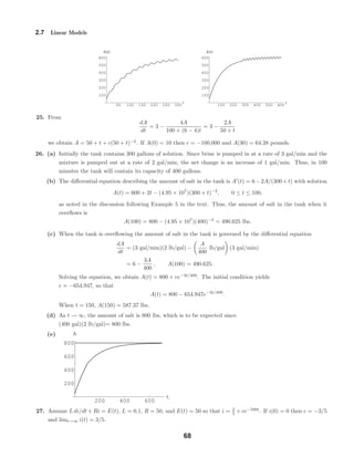
46. 2.7 Linear Models
Thus
d
dt
[e0.1t
T] = 10e0.1t
− 4
e0.1t
T = 100e0.1t
− 4t + c
and
T(t) = 100 − 4te−0.1t
+ ce−0.1t
.
Now T(0) = 80 so 100 + c = 80, c = −20 and
T(t) = 100 − 4te−0.1t
− 20e−0.1t
= 100 − (4t + 20)e−0.1t
.
The thinner curve verifies the prediction of cooling followed by warming toward 100◦
. The wider curve shows
the temperature Tm of the liquid bath.
19. From dA/dt = 4 − A/50 we obtain A = 200 + ce−t/50
. If A(0) = 30 then c = −170 and
A = 200 − 170e−t/50
.
20. From dA/dt = 0 − A/50 we obtain A = ce−t/50
. If A(0) = 30 then c = 30 and A = 30e−t/50
.
21. From dA/dt = 10 − A/100 we obtain A = 1000 + ce−t/100
. If A(0) = 0 then c = −1000 and A(t) =
1000 − 1000e−t/100
.
22. From Problem 21 the number of pounds of salt in the tank at time t is A(t) = 1000 − 1000e−t/100
. The
concentration at time t is c(t) = A(t)/500 = 2 − 2e−t/100
. Therefore c(5) = 2 − 2e−1/20
= 0.0975 lb/gal and
limt→∞ c(t) = 2. Solving c(t) = 1 = 2 − 2e−t/100
for t we obtain t = 100 ln 2 ≈ 69.3 min.
23. From
dA
dt
= 10 −
10A
500 − (10 − 5)t
= 10 −
2A
100 − t
we obtain A = 1000 − 10t + c(100 − t)2
. If A(0) = 0 then c = − 1
10 . The tank is empty in 100 minutes.
24. With cin(t) = 2 + sin(t/4) lb/gal, the initial-value problem is
dA
dt
+
1
100
A = 6 + 3 sin
t
4
, A(0) = 50.
The differential equation is linear with integrating factor e dt/100
= et/100
, so
d
dt
[et/100
A(t)] = 6 + 3 sin
t
4
et/100
et/100
A(t) = 600et/100
+
150
313
et/100
sin
t
4
−
3750
313
et/100
cos
t
4
+ c,
and
A(t) = 600 +
150
313
sin
t
4
−
3750
313
cos
t
4
+ ce−t/100
.
Letting t = 0 and A = 50 we have 600 − 3750/313 + c = 50 and c = −168400/313. Then
A(t) = 600 +
150
313
sin
t
4
−
3750
313
cos
t
4
−
168400
313
e−t/100
.
The graphs on [0, 300] and [0, 600] below show the effect of the sine function in the input when compared with
the graph in Figure 2.38(a) in the text.
67

47. 50 100 150 200 250 300
t
100
200
300
400
500
600
A t
100 200 300 400 500 600
t
100
200
300
400
500
600
A t
200 400 600
t
200
400
600
800
A
2.7 Linear Models
25. From
dA
dt
= 3 −
4A
100 + (6 − 4)t
= 3 −
2A
50 + t
we obtain A = 50 + t + c(50 + t)−2
. If A(0) = 10 then c = −100,000 and A(30) = 64.38 pounds.
26. (a) Initially the tank contains 300 gallons of solution. Since brine is pumped in at a rate of 3 gal/min and the
mixture is pumped out at a rate of 2 gal/min, the net change is an increase of 1 gal/min. Thus, in 100
minutes the tank will contain its capacity of 400 gallons.
(b) The differential equation describing the amount of salt in the tank is A (t) = 6−2A/(300+t) with solution
A(t) = 600 + 2t − (4.95 × 107
)(300 + t)−2
, 0 ≤ t ≤ 100,
as noted in the discussion following Example 5 in the text. Thus, the amount of salt in the tank when it
overflows is
A(100) = 800 − (4.95 × 107
)(400)−2
= 490.625 lbs.
(c) When the tank is overflowing the amount of salt in the tank is governed by the differential equation
dA
dt
= (3 gal/min)(2 lb/gal) −
A
400
lb/gal (3 gal/min)
= 6 −
3A
400
, A(100) = 490.625.
Solving the equation, we obtain A(t) = 800 + ce−3t/400
. The initial condition yields
c = −654.947, so that
A(t) = 800 − 654.947e−3t/400
.
When t = 150, A(150) = 587.37 lbs.
(d) As t → ∞, the amount of salt is 800 lbs, which is to be expected since
(400 gal)(2 lb/gal)= 800 lbs.
(e)
27. Assume L di/dt + Ri = E(t), L = 0.1, R = 50, and E(t) = 50 so that i = 3
5 + ce−500t
. If i(0) = 0 then c = −3/5
and limt→∞ i(t) = 3/5.
68

48. 2.7 Linear Models
28. Assume L di/dt + Ri = E(t), E(t) = E0 sin ωt, and i(0) = i0 so that
i =
E0R
L2ω2 + R2
sin ωt −
E0Lω
L2ω2 + R2
cos ωt + ce−Rt/L
.
Since i(0) = i0 we obtain c = i0 +
E0Lω
L2ω2 + R2
.
29. Assume R dq/dt + (1/C)q = E(t), R = 200, C = 10−4
, and E(t) = 100 so that q = 1/100 + ce−50t
. If q(0) = 0
then c = −1/100 and i = 1
2 e−50t
.
30. Assume R dq/dt + (1/C)q = E(t), R = 1000, C = 5 × 10−6
, and E(t) = 200. Then q = 1
1000 + ce−200t
and
i = −200ce−200t
. If i(0) = 0.4 then c = − 1
500 , q(0.005) = 0.003 coulombs, and i(0.005) = 0.1472 amps. We have
q → 1
1000 as t → ∞.
31. For 0 ≤ t ≤ 20 the differential equation is 20 di/dt + 2i = 120. An integrating factor is et/10
, so (d/dt)[et/10
i] =
6et/10
and i = 60 + c1e−t/10
. If i(0) = 0 then c1 = −60 and i = 60 − 60e−t/10
. For t > 20 the differential
equation is 20 di/dt + 2i = 0 and i = c2e−t/10
. At t = 20 we want c2e−2
= 60 − 60e−2
so that c2 = 60 e2
− 1 .
Thus
i(t) =
60 − 60e−t/10
, 0 ≤ t ≤ 20
60 e2
− 1 e−t/10
, t > 20.
32. Separating variables, we obtain
dq
E0 − q/C
=
dt
k1 + k2t
−C ln E0 −
q
C
=
1
k2
ln |k1 + k2t| + c1
(E0 − q/C)−C
(k1 + k2t)1/k2
= c2.
Setting q(0) = q0 we find c2 = (E0 − q0/C)−C
/k
1/k2
1 , so
(E0 − q/C)−C
(k1 + k2t)1/k2
=
(E0 − q0/C)−C
k
1/k2
1
E0 −
q
C
−C
= E0 −
q0
C
−C k1
k + k2t
−1/k2
E0 −
q
C
= E0 −
q0
C
k1
k + k2t
1/Ck2
q = E0C + (q0 − E0C)
k1
k + k2t
1/Ck2
.
33. (a) From m dv/dt = mg − kv we obtain v = mg/k + ce−kt/m
. If v(0) = v0 then c = v0 − mg/k and the solution
of the initial-value problem is
v(t) =
mg
k
+ v0 −
mg
k
e−kt/m
.
(b) As t → ∞ the limiting velocity is mg/k.
(c) From ds/dt = v and s(0) = 0 we obtain
s(t) =
mg
k
t −
m
k
v0 −
mg
k
e−kt/m
+
m
k
v0 −
mg
k
.
34. (a) Integrating d2
s/dt2
= −g we get v(t) = ds/dt = −gt + c. From v(0) = 300 we find c = 300, and we are
given g = 32, so the velocity is v(t) = −32t + 300.
69

49. 2.7 Linear Models
(b) Integrating again and using s(0) = 0 we get s(t) = −16t2
+ 300t. The maximum height is attained when
v = 0, that is, at ta = 9.375. The maximum height will be s(9.375) = 1406.25 ft.
35. When air resistance is proportional to velocity, the model for the velocity is m dv/dt = −mg − kv (using the
fact that the positive direction is upward.) Solving the differential equation using separation of variables we
obtain v(t) = −mg/k + ce−kt/m
. From v(0) = 300 we get
v(t) = −
mg
k
+ 300 +
mg
k
e−kt/m
.
Integrating and using s(0) = 0 we find
s(t) = −
mg
k
t +
m
k
300 +
mg
k
(1 − e−kt/m
).
Setting k = 0.0025, m = 16/32 = 0.5, and g = 32 we have
s(t) = 1,340,000 − 6,400t − 1,340,000e−0.005t
and
v(t) = −6,400 + 6,700e−0.005t
.
The maximum height is attained when v = 0, that is, at ta = 9.162. The maximum height will be s(9.162) =
1363.79 ft, which is less than the maximum height in Problem 34.
36. Assuming that the air resistance is proportional to velocity and the positive direction is downward with s(0) = 0,
the model for the velocity is m dv/dt = mg − kv. Using separation of variables to solve this differential
equation, we obtain v(t) = mg/k + ce−kt/m
. Then, using v(0) = 0, we get v(t) = (mg/k)(1 − e−kt/m
).
Letting k = 0.5, m = (125 + 35)/32 = 5, and g = 32, we have v(t) = 320(1 − e−0.1t
). Integrating,
we find s(t) = 320t + 3200e−0.1t
+ c1. Solving s(0) = 0 for c1 we find c1 = −3200, therefore s(t) =
320t + 3200e−0.1t
− 3200. At t = 15, when the parachute opens, v(15) = 248.598 and s(15) = 2314.02.
At this time the value of k changes to k = 10 and the new initial velocity is v0 = 248.598. With the parachute
open, the skydiver’s velocity is vp(t) = mg/k + c2e−kt/m
, where t is reset to 0 when the parachute opens.
Letting m = 5, g = 32, and k = 10, this gives vp(t) = 16 + c2e−2t
. From v(0) = 248.598 we find c2 = 232.598,
so vp(t) = 16 + 232.598e−2t
. Integrating, we get sp(t) = 16t − 116.299e−2t
+ c3. Solving sp(0) = 0 for c3,
we find c3 = 116.299, so sp(t) = 16t − 116.299e−2t
+ 116.299. Twenty seconds after leaving the plane is five
seconds after the parachute opens. The skydiver’s velocity at this time is vp(5) = 16.0106 ft/s and she has
fallen a total of s(15) + sp(5) = 2314.02 + 196.294 = 2510.31 ft. Her terminal velocity is limt→∞ vp(t) = 16, so
she has very nearly reached her terminal velocity five seconds after the parachute opens. When the parachute
opens, the distance to the ground is 15,000 − s(15) = 15,000 − 2,314 = 12,686 ft. Solving sp(t) = 12,686 we
get t = 785.6 s = 13.1 min. Thus, it will take her approximately 13.1 minutes to reach the ground after her
parachute has opened and a total of (785.6 + 15)/60 = 13.34 minutes after she exits the plane.
37. (a) The differential equation is first-order and linear. Letting b = k/ρ, the integrating factor is e 3b dt/(bt+r0)
=
(r0 + bt)3
. Then
d
dt
[(r0 + bt)3
v] = g(r0 + bt)3
and (r0 + bt)3
v =
g
4b
(r0 + bt)4
+ c.
The solution of the differential equation is v(t) = (g/4b)(r0 + bt) + c(r0 + bt)−3
. Using v(0) = 0 we find
c = −gr4
0/4b, so that
v(t) =
g
4b
(r0 + bt) −
gr4
0
4b(r0 + bt)3
=
gρ
4k
r0 +
k
ρ
t −
gρr4
0
4k(r0 + kt/ρ)3
.
(b) Integrating dr/dt = k/ρ we get r = kt/ρ + c. Using r(0) = r0 we have c = r0, so r(t) = kt/ρ + r0.
70

50. M k1
k1 k2
A
r
k
x
2.7 Linear Models
(c) If r = 0.007 ft when t = 10 s, then solving r(10) = 0.007 for k/ρ, we obtain k/ρ = −0.0003 and r(t) =
0.01 − 0.0003t. Solving r(t) = 0 we get t = 33.3, so the raindrop will have evaporated completely at
33.3 seconds.
38. Separating variables, we obtain dP/P = k cos t dt, so
ln |P| = k sin t + c and P = c1ek sin t
.
If P(0) = P0, then c1 = P0 and P = P0ek sin t
.
39. (a) From dP/dt = (k1 − k2)P we obtain P = P0e(k1−k2)t
where P0 = P(0).
(b) If k1 > k2 then P → ∞ as t → ∞. If k1 = k2 then P = P0 for every t. If k1 < k2 then P → 0 as t → ∞.
40. (a) Solving k1(M − A) − k2A = 0 for A we find the equilibrium solution
A = k1M/(k1 +k2). From the phase portrait we see that limt→∞ A(t) = k1M/(k1 +k2).
Since k2 > 0, the material will never be completely memorized and the larger k2 is, the
less the amount of material will be memorized over time.
(b) Write the differential equation in the form dA/dt+(k1 +k2)A = k1M.
Then an integrating factor is e(k1+k2)t
, and
d
dt
e(k1+k2)t
A = k1Me(k1+k2)t
e(k1+k2)t
A =
k1M
k1 + k2
e(k1+k2)t
+ c
A =
k1M
k1 + k2
+ ce−(k1+k2)t
.
Using A(0) = 0 we find c = −
k1M
k1 + k2
and A =
k1M
k1 + k2
1 − e−(k1+k2)t
. As t → ∞,
A →
k1M
k1 + k2
.
41. (a) Solving r−kx = 0 for x we find the equilibrium solution x = r/k. When x < r/k, dx/dt > 0
and when x > r/k, dx/dt < 0. From the phase portrait we see that limt→∞ x(t) = r/k.
71

51. t
rêk
x
4 6 10 12 16 18 22 24
t
5
10
E
2.7 Linear Models
(b) From dx/dt = r − kx and x(0) = 0 we obtain x = r/k − (r/k)e−kt
so that
x → r/k as t → ∞. If x(T) = r/2k then T = (ln 2)/k.
42. The bar removed from the oven has an initial temperature of 300◦
F and, after being removed from the oven,
approaches a temperature of 70◦
F. The bar taken from the room and placed in the oven has an initial temperature
of 70◦
F and approaches a temperature of 300◦
F in the oven. Since the two temperature functions are continuous
they must intersect at some time, t∗
.
43. (a) For 0 ≤ t < 4, 6 ≤ t < 10 and 12 ≤ t < 16, no voltage is applied to the heart and E(t) = 0. At the other
times, the differential equation is dE/dt = −E/RC. Separating variables, integrating, and solving for e,
we get E = ke−t/RC
, subject to E(4) = E(10) = E(16) = 12. These intitial conditions yield, respectively,
k = 12e4/RC
, k = 12e10/RC
, k = 12e16/RC
, and k = 12e22/RC
. Thus
E(t) =



0, 0 ≤ t < 4, 6 ≤ t < 10, 12 ≤ t < 16
12e(4−t)/RC
, 4 ≤ t < 6
12e(10−t)/RC
, 10 ≤ t < 12
12e(16−t)/RC
, 16 ≤ t < 18
12e(22−t)/RC
, 22 ≤ t < 24.
(b)
44. (a) (i) Using Newton’s second law of motion, F = ma = m dv/dt, the differential equation for the velocity v is
m
dv
dt
= mg sin θ or
dv
dt
= g sin θ,
where mg sin θ, 0 < θ < π/2, is the component of the weight along the plane in the direction of motion.
(ii) The model now becomes
m
dv
dt
= mg sin θ − µmg cos θ,
where µmg cos θ is the component of the force of sliding friction (which acts perpendicular to the plane)
along the plane. The negative sign indicates that this component of force is a retarding force which acts in
the direction opposite to that of motion.
(iii) If air resistance is taken to be proportional to the instantaneous velocity of the body, the model becomes
m
dv
dt
= mg sin θ − µmg cos θ − kv,
where k is a constant of proportionality.
72

52. 2.7 Linear Models
(b) (i) With m = 3 slugs, the differential equation is
3
dv
dt
= (96) ·
1
2
or
dv
dt
= 16.
Integrating the last equation gives v(t) = 16t + c1. Since v(0) = 0, we have c1 = 0 and so v(t) = 16t.
(ii) With m = 3 slugs, the differential equation is
3
dv
dt
= (96) ·
1
2
−
√
3
4
· (96) ·
√
3
2
or
dv
dt
= 4.
In this case v(t) = 4t.
(iii) When the retarding force due to air resistance is taken into account, the differential equation for
velocity v becomes
3
dv
dt
= (96) ·
1
2
−
√
3
4
· (96) ·
√
3
2
−
1
4
v or 3
dv
dt
= 12 −
1
4
v.
The last differential equation is linear and has solution v(t) = 48 + c1e−t/12
. Since v(0) = 0, we find
c1 = −48, so v(t) = 48 − 48e−t/12
.
45. (a) (i) If s(t) is distance measured down the plane from the highest point, then ds/dt = v. Integrating
ds/dt = 16t gives s(t) = 8t2
+ c2. Using s(0) = 0 then gives c2 = 0. Now the length L of the plane is
L = 50/ sin 30◦
= 100 ft. The time it takes the box to slide completely down the plane is the solution of
s(t) = 100 or t2
= 25/2, so t ≈ 3.54 s.
(ii) Integrating ds/dt = 4t gives s(t) = 2t2
+ c2. Using s(0) = 0 gives c2 = 0, so s(t) = 2t2
and the solution
of s(t) = 100 is now t ≈ 7.07 s.
(iii) Integrating ds/dt = 48 − 48e−t/12
and using s(0) = 0 to determine the constant of integration, we
obtain s(t) = 48t + 576e−t/12
− 576. With the aid of a CAS we find that the solution of s(t) = 100, or
100 = 48t + 576e−t/12
− 576 or 0 = 48t + 576e−t/12
− 676,
is now t ≈ 7.84 s.
(b) The differential equation m dv/dt = mg sin θ − µmg cos θ can be written
m
dv
dt
= mg cos θ(tan θ − µ).
If tan θ = µ, dv/dt = 0 and v(0) = 0 implies that v(t) = 0. If tan θ < µ and v(0) = 0, then integration
implies v(t) = g cos θ(tan θ − µ)t < 0 for all time t.
(c) Since tan 23◦
= 0.4245 and µ =
√
3/4 = 0.4330, we see that tan 23◦
< 0.4330. The differential equation
is dv/dt = 32 cos 23◦
(tan 23◦
−
√
3/4) = −0.251493. Integration and the use of the initial condition gives
v(t) = −0.251493t + 1. When the box stops, v(t) = 0 or 0 = −0.251493t + 1 or t = 3.976254 s. From
s(t) = −0.125747t2
+ t we find s(3.976254) = 1.988119 ft.
(d) With v0 > 0, v(t) = −0.251493t + v0 and s(t) = −0.125747t2
+ v0t. Because two real positive solutions
of the equation s(t) = 100, or 0 = −0.125747t2
+ v0t − 100, would be physically meaningless, we use
the quadratic formula and require that b2
− 4ac = 0 or v2
0 − 50.2987 = 0. From this last equality we
find v0 ≈ 7.092164 ft/s. For the time it takes the box to traverse the entire inclined plane, we must
have 0 = −0.125747t2
+ 7.092164t − 100. Mathematica gives complex roots for the last equation: t =
28.2001 ± 0.0124458i. But, for
0 = −0.125747t2
+ 7.092164691t − 100,
73

53. 0
2000
N
5 10 15 20
t
500
1000
1500
2000
N
2.7 Linear Models
the roots are t = 28.1999 s and t = 28.2004 s. So if v0 > 7.092164, we are guaranteed that the box will slide
completely down the plane.
46. (a) We saw in part (b) of Problem 34 that the ascent time is ta = 9.375. To find when the cannonball hits the
ground we solve s(t) = −16t2
+ 300t = 0, getting a total time in flight of t = 18.75 s. Thus, the time of
descent is td = 18.75 − 9.375 = 9.375. The impact velocity is vi = v(18.75) = −300, which has the same
magnitude as the initial velocity.
(b) We saw in Problem 35 that the ascent time in the case of air resistance is ta = 9.162. Solving s(t) =
1,340,000 − 6,400t − 1,340,000e−0.005t
= 0 we see that the total time of flight is 18.466 s. Thus, the descent
time is td = 18.466 − 9.162 = 9.304. The impact velocity is vi = v(18.466) = −290.91, compared to an
initial velocity of v0 = 300.
EXERCISES 2.8
Nonlinear Models
1. (a) Solving N(1 − 0.0005N) = 0 for N we find the equilibrium solutions N = 0 and N = 2000.
When 0 < N < 2000, dN/dt > 0. From the phase portrait we see that limt→∞ N(t) = 2000.
A graph of the solution is shown in part (b).
(b) Separating variables and integrating we have
dN
N(1 − 0.0005N)
=
1
N
−
1
N − 2000
dN = dt
and
ln N − ln(N − 2000) = t + c.
Solving for N we get N(t) = 2000ec+t
/(1 + ec+t
) = 2000ec
et
/(1 + ec
et
). Using N(0) = 1 and solving for
ec
we find ec
= 1/1999 and so N(t) = 2000et
/(1999 + et
). Then N(10) = 1833.59, so 1834 companies are
expected to adopt the new technology when t = 10.
2. From dN/dt = N(a − bN) and N(0) = 500 we obtain
N =
500a
500b + (a − 500b)e−at
.
Since limt→∞ N = a/b = 50,000 and N(1) = 1000 we have a = 0.7033, b = 0.00014, and N =
50,000/(1 + 99e−0.7033t
) .
74

54. Census Predicted %
Year Population Population Error Error
1790 3.929 3.929 0.000 0.00
1800 5.308 5.334 -0.026 -0.49
1810 7.240 7.222 0.018 0.24
1820 9.638 9.746 -0.108 -1.12
1830 12.866 13.090 -0.224 -1.74
1840 17.069 17.475 -0.406 -2.38
1850 23.192 23.143 0.049 0.21
1860 31.433 30.341 1.092 3.47
1870 38.558 39.272 -0.714 -1.85
1880 50.156 50.044 0.112 0.22
1890 62.948 62.600 0.348 0.55
1900 75.996 76.666 -0.670 -0.88
1910 91.972 91.739 0.233 0.25
1920 105.711 107.143 -1.432 -1.35
1930 122.775 122.140 0.635 0.52
1940 131.669 136.068 -4.399 -3.34
1950 150.697 148.445 2.252 1.49
2.8 Nonlinear Models
3. From dP/dt = P 10−1
− 10−7
P and P(0) = 5000 we obtain P = 500/(0.0005 + 0.0995e−0.1t
) so that
P → 1,000,000 as t → ∞. If P(t) = 500,000 then t = 52.9 months.
4. (a) We have dP/dt = P(a − bP) with P(0) = 3.929 million. Using separation of variables we obtain
P(t) =
3.929a
3.929b + (a − 3.929b)e−at
=
a/b
1 + (a/3.929b − 1)e−at
=
c
1 + (c/3.929 − 1)e−at
,
where c = a/b. At t = 60(1850) the population is 23.192 million, so
23.192 =
c
1 + (c/3.929 − 1)e−60a
or c = 23.192 + 23.192(c/3.929 − 1)e−60a
. At t = 120(1910),
91.972 =
c
1 + (c/3.929 − 1)e−120a
or c = 91.972 + 91.972(c/3.929 − 1)(e−60a
)2
. Combining the two equations for c we get
(c − 23.192)/23.192
c/3.929 − 1
2
c
3.929
− 1 =
c − 91.972
91.972
or
91.972(3.929)(c − 23.192)2
= (23.192)2
(c − 91.972)(c − 3.929).
The solution of this quadratic equation is c = 197.274. This in turn gives a = 0.0313. Therefore,
P(t) =
197.274
1 + 49.21e−0.0313t
.
(b)
The model predicts a population of 159.0 million for 1960 and 167.8 million for 1970. The census populations
for these years were 179.3 and 203.3, respectively. The percentage errors are 12.8 and 21.2, respectively.
75

55. 1
4
P
t
P
3
1
4
2.8 Nonlinear Models
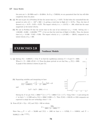
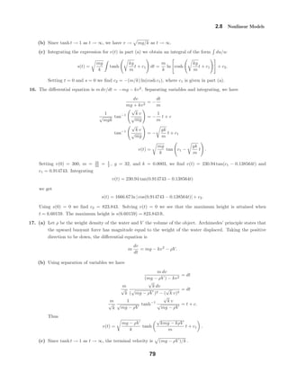
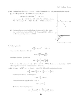
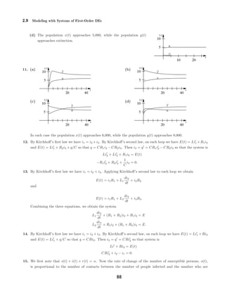
5. (a) The differential equation is dP/dt = P(5 − P) − 4. Solving P(5 − P) − 4 = 0 for P we
obtain equilibrium solutions P = 1 and P = 4. The phase portrait is shown on the right and
solution curves are shown in part (b). We see that for P0 > 4 and 1 < P0 < 4 the population
approaches 4 as t increases. For 0 < P < 1 the population decreases to 0 in finite time.
(b) The differential equation is
dP
dt
= P(5 − P) − 4 = −(P2
− 5P + 4) = −(P − 4)(P − 1).
Separating variables and integrating, we obtain
dP
(P − 4)(P − 1)
= −dt
1/3
P − 4
−
1/3
P − 1
dP = −dt
1
3
ln
P − 4
P − 1
= −t + c
P − 4
P − 1
= c1e−3t
.
Setting t = 0 and P = P0 we find c1 = (P0 − 4)/(P0 − 1). Solving for P we obtain
P(t) =
4(P0 − 1) − (P0 − 4)e−3t
(P0 − 1) − (P0 − 4)e−3t
.
(c) To find when the population becomes extinct in the case 0 < P0 < 1 we set P = 0 in
P − 4
P − 1
=
P0 − 4
P0 − 1
e−3t
from part (a) and solve for t. This gives the time of extinction
t = −
1
3
ln
4(P0 − 1)
P0 − 4
.
6. Solving P(5 − P) − 25
4 = 0 for P we obtain the equilibrium solution P = 5
2 . For P = 5
2 , dP/dt < 0. Thus,
if P0 < 5
2 , the population becomes extinct (otherwise there would be another equilibrium solution.) Using
separation of variables to solve the initial-value problem, we get
P(t) = [4P0 + (10P0 − 25)t]/[4 + (4P0 − 10)t].
To find when the population becomes extinct for P0 < 5
2 we solve P(t) = 0 for t. We see that the time of
extinction is t = 4P0/5(5 − 2P0).
7. Solving P(5−P)−7 = 0 for P we obtain complex roots, so there are no equilibrium solutions. Since dP/dt < 0
for all values of P, the population becomes extinct for any initial condition. Using separation of variables to
solve the initial-value problem, we get
P(t) =
5
2
+
√
3
2
tan tan−1 2P0 − 5
√
3
−
√
3
2
t .
76

56. t
e
P
t
1êe
P
500 1000 1500
t
2
4
6
8
10
h
2.8 Nonlinear Models
Solving P(t) = 0 for t we see that the time of extinction is
t =
2
3
√
3 tan−1
(5/
√
3 ) +
√
3 tan−1
(2P0 − 5)/
√
3 .
8. (a) The differential equation is dP/dt = P(1 − ln P), which has the equilibrium
solution P = e. When P0 > e, dP/dt < 0, and when P0 < e, dP/dt > 0.
(b) The differential equation is dP/dt = P(1 + ln P), which has the equilibrium
solution P = 1/e. When P0 > 1/e, dP/dt > 0, and when P0 < 1/e, dP/dt < 0.
(c) From dP/dt = P(a − b ln P) we obtain −(1/b) ln |a − b ln P| = t + c1 so that P = ea/b
e−ce−bt
. If P(0) = P0
then c = (a/b) − ln P0.
9. Let X = X(t) be the amount of C at time t and dX/dt = k(120 − 2X)(150 − X). If X(0) = 0 and X(5) = 10,
then
X(t) =
150 − 150e180kt
1 − 2.5e180kt
,
where k = .0001259 and X(20) = 29.3 grams. Now by L’Hˆopital’s rule, X → 60 as t → ∞, so that the amount
of A → 0 and the amount of B → 30 as t → ∞.
10. From dX/dt = k(150 − X)2
, X(0) = 0, and X(5) = 10 we obtain X = 150 − 150/(150kt + 1) where
k = .000095238. Then X(20) = 33.3 grams and X → 150 as t → ∞ so that the amount of A → 0 and
the amount of B → 0 as t → ∞. If X(t) = 75 then t = 70 minutes.
11. (a) The initial-value problem is dh/dt = −8Ah
√
h /Aw, h(0) = H.
Separating variables and integrating we have
dh
√
h
= −
8Ah
Aw
dt and 2
√
h = −
8Ah
Aw
t + c.
Using h(0) = H we find c = 2
√
H , so the solution of the
initial-value problem is h(t) = (Aw
√
H − 4Aht)/Aw, where
Aw
√
H − 4Aht ≥ 0. Thus,
h(t) = (Aw
√
H − 4Aht)2
/A2
w for 0 ≤ t ≤ AwH/4Ah.
(b) Identifying H = 10, Aw = 4π, and Ah = π/576 we have h(t) = t2
/331,776 − ( 5/2 /144)t + 10. Solving
h(t) = 0 we see that the tank empties in 576
√
10 seconds or 30.36 minutes.
12. To obtain the solution of this differential equation we use h(t) from Problem 13 in Exercises 1.3. Then
h(t) = (Aw
√
H − 4cAht)2
/A2
w. Solving h(t) = 0 with c = 0.6 and the values from Problem 11 we see that
the tank empties in 3035.79 seconds or 50.6 minutes.
77

57. 2.8 Nonlinear Models
13. (a) Separating variables and integrating gives
6h3/2
dh = −5t and
12
5
h5/2
= −5t + c.
Using h(0) = 20 we find c = 1920
√
5 , so the solution of the initial-value problem is h(t) = 800
√
5− 25
12 t
2/5
.
Solving h(t) = 0 we see that the tank empties in 384
√
5 seconds or 14.31 minutes.
(b) When the height of the water is h, the radius of the top of the water is r = h tan 30◦
= h/
√
3 and
Aw = πh2
/3. The differential equation is
dh
dt
= −c
Ah
Aw
2gh = −0.6
π(2/12)2
πh2/3
√
64h = −
2
5h3/2
.
Separating variables and integrating gives
5h3/2
dh = −2 dt and 2h5/2
= −2t + c.
Using h(0) = 9 we find c = 486, so the solution of the initial-value problem is h(t) = (243 − t)2/5
. Solving
h(t) = 0 we see that the tank empties in 24.3 seconds or 4.05 minutes.
14. When the height of the water is h, the radius of the top of the water is 2
5 (20 − h) and
Aw = 4π(20 − h)2
/25. The differential equation is
dh
dt
= −c
Ah
Aw
2gh = −0.6
π(2/12)2
4π(20 − h)2/25
√
64h = −
5
6
√
h
(20 − h)2
.
Separating variables and integrating we have
(20 − h)2
√
h
dh = −
5
6
dt and 800
√
h −
80
3
h3/2
+
2
5
h5/2
= −
5
6
t + c.
Using h(0) = 20 we find c = 2560
√
5/3, so an implicit solution of the initial-value problem is
800
√
h −
80
3
h3/2
+
2
5
h5/2
= −
5
6
t +
2560
√
5
3
.
To find the time it takes the tank to empty we set h = 0 and solve for t. The tank empties in 1024
√
5 seconds
or 38.16 minutes. Thus, the tank empties more slowly when the base of the cone is on the bottom.
15. (a) After separating variables we obtain
m dv
mg − kv2
= dt
1
g
dv
1 − (
√
k v/
√
mg )2
= dt
√
mg
√
k g
k/mg dv
1 − (
√
k v/
√
mg )2
= dt
m
kg
tanh−1
√
k v
√
mg
= t + c
tanh−1
√
k v
√
mg
=
kg
m
t + c1.
Thus the velocity at time t is
v(t) =
mg
k
tanh
kg
m
t + c1 .
Setting t = 0 and v = v0 we find c1 = tanh−1
(
√
k v0/
√
mg ).
78

58. 2.8 Nonlinear Models
(b) Since tanh t → 1 as t → ∞, we have v → mg/k as t → ∞.
(c) Integrating the expression for v(t) in part (a) we obtain an integral of the form du/u:
s(t) =
mg
k
tanh
kg
m
t + c1 dt =
m
k
ln cosh
kg
m
t + c1 + c2.
Setting t = 0 and s = 0 we find c2 = −(m/k) ln(cosh c1), where c1 is given in part (a).
16. The differential equation is m dv/dt = −mg − kv2
. Separating variables and integrating, we have
dv
mg + kv2
= −
dt
m
1
√
mgk
tan−1
√
k v
√
mg
= −
1
m
t + c
tan−1
√
k v
√
mg
= −
gk
m
t + c1
v(t) =
mg
k
tan c1 −
gk
m
t .
Setting v(0) = 300, m = 16
32 = 1
2 , g = 32, and k = 0.0003, we find v(t) = 230.94 tan(c1 − 0.138564t) and
c1 = 0.914743. Integrating
v(t) = 230.94 tan(0.914743 − 0.138564t)
we get
s(t) = 1666.67 ln | cos(0.914743 − 0.138564t)| + c2.
Using s(0) = 0 we find c2 = 823.843. Solving v(t) = 0 we see that the maximum height is attained when
t = 6.60159. The maximum height is s(6.60159) = 823.843 ft.
17. (a) Let ρ be the weight density of the water and V the volume of the object. Archimedes’ principle states that
the upward buoyant force has magnitude equal to the weight of the water displaced. Taking the positive
direction to be down, the differential equation is
m
dv
dt
= mg − kv2
− ρV.
(b) Using separation of variables we have
m dv
(mg − ρV ) − kv2
= dt
m
√
k
√
k dv
(
√
mg − ρV )2 − (
√
k v)2
= dt
m
√
k
1
√
mg − ρV
tanh−1
√
k v
√
mg − ρV
= t + c.
Thus
v(t) =
mg − ρV
k
tanh
√
kmg − kρV
m
t + c1 .
(c) Since tanh t → 1 as t → ∞, the terminal velocity is (mg − ρV )/k .
79

59. 2.8 Nonlinear Models
18. (a) Writing the equation in the form (x − x2 + y2 )dx + y dy = 0 we identify M = x − x2 + y2 and N = y.
Since M and N are both homogeneous functions of degree 1 we use the substitution y = ux. It follows that
x − x2 + u2x2 dx + ux(u dx + x du) = 0
x 1 − 1 + u2 + u2
dx + x2
u du = 0
−
u du
1 + u2 −
√
1 + u2
=
dx
x
u du
√
1 + u2 (1 −
√
1 + u2 )
=
dx
x
.
Letting w = 1 −
√
1 + u2 we have dw = −u du/
√
1 + u2 so that
− ln 1 − 1 + u2 = ln |x| + c
1
1 −
√
1 + u2
= c1x
1 − 1 + u2 = −
c2
x
(−c2 = 1/c1)
1 +
c2
x
= 1 +
y2
x2
1 +
2c2
x
+
c2
2
x2
= 1 +
y2
x2
.
Solving for y2
we have
y2
= 2c2x + c2
2 = 4
c2
2
x +
c2
2
which is a family of parabolas symmetric with respect to the x-axis with vertex at (−c2/2, 0) and focus at
the origin.
(b) Let u = x2
+ y2
so that
du
dx
= 2x + 2y
dy
dx
.
Then
y
dy
dx
=
1
2
du
dx
− x
and the differential equation can be written in the form
1
2
du
dx
− x = −x +
√
u or
1
2
du
dx
=
√
u .
Separating variables and integrating gives
du
2
√
u
= dx
√
u = x + c
u = x2
+ 2cx + c2
x2
+ y2
= x2
+ 2cx + c2
y2
= 2cx + c2
.
19. (a) From 2W2
− W3
= W2
(2 − W) = 0 we see that W = 0 and W = 2 are constant solutions.
80

60. x
W
−3 3
2
2000 4000 6000 8000 10000
t
2
4
6
8
10
h
2.8 Nonlinear Models
(b) Separating variables and using a CAS to integrate we get
dW
W
√
4 − 2W
= dx and − tanh−1 1
2
√
4 − 2W = x + c.
Using the facts that the hyperbolic tangent is an odd function and 1 − tanh2
x = sech2
x we have
1
2
√
4 − 2W = tanh(−x − c) = − tanh(x + c)
1
4
(4 − 2W) = tanh2
(x + c)
1 −
1
2
W = tanh2
(x + c)
1
2
W = 1 − tanh2
(x + c) = sech2
(x + c).
Thus, W(x) = 2 sech2
(x + c).
(c) Letting x = 0 and W = 2 we find that sech2
(c) = 1 and c = 0.
20. (a) Solving r2
+ (10 − h)2
= 102
for r2
we see that r2
= 20h − h2
. Combining the rate of input of water, π,
with the rate of output due to evaporation, kπr2
= kπ(20h−h2
), we have dV/dt = π −kπ(20h−h2
). Using
V = 10πh2
− 1
3 πh3
, we see also that dV/dt = (20πh − πh2
)dh/dt. Thus,
(20πh − πh2
)
dh
dt
= π − kπ(20h − h2
) and
dh
dt
=
1 − 20kh + kh2
20h − h2
.
(b) Letting k = 1/100, separating variables and integrating (with the help
of a CAS), we get
100h(h − 20)
(h − 10)2
dh = dt and
100(h2
− 10h + 100)
10 − h
= t + c.
Using h(0) = 0 we find c = 1000, and solving for h we get h(t) =
0.005
√
t2 + 4000t−t , where the positive square root is chosen because
h ≥ 0.
(c) The volume of the tank is V = 2
3 π(10)3
feet, so at a rate of π cubic feet per minute, the tank will fill in
2
3 (10)3
≈ 666.67 minutes ≈ 11.11 hours.
(d) At 666.67 minutes, the depth of the water is h(666.67) = 5.486 feet. From the graph in (b) we suspect that
limt→∞ h(t) = 10, in which case the tank will never completely fill. To prove this we compute the limit of
h(t):
lim
t→∞
h(t) = 0.005 lim
t→∞
t2 + 4000t − t = 0.005 lim
t→∞
t2
+ 4000t − t2
√
t2 + 4000t + t
= 0.005 lim
t→∞
4000t
t 1 + 4000/t + t
= 0.005
4000
1 + 1
= 0.005(2000) = 10.
81

61. t P(t) Q(t)
0 3.929 0.035
10 5.308 0.036
20 7.240 0.033
30 9.638 0.033
40 12.866 0.033
50 17.069 0.036
60 23.192 0.036
70 31.433 0.023
80 38.558 0.030
90 50.156 0.026
100 62.948 0.021
110 75.996 0.021
120 91.972 0.015
130 105.711 0.016
140 122.775 0.007
150 131.669 0.014
160 150.697 0.019
170 179.300
20 40 60 80 100 120 140
P
0.005
0.01
0.015
0.02
0.025
0.03
0.035
Q
25 50 75 100 125 150
t
25
50
75
100
125
150
175
P
2.8 Nonlinear Models
21. (a)
(b) The regression line is Q = 0.0348391 − 0.000168222P.
(c) The solution of the logistic equation is given in equation (5) in the text. Identifying a = 0.0348391 and
b = 0.000168222 we have
P(t) =
aP0
bP0 + (a − bP0)e−at
.
(d) With P0 = 3.929 the solution becomes
P(t) =
0.136883
0.000660944 + 0.0341781e−0.0348391t
.
(e)
(f) We identify t = 180 with 1970, t = 190 with 1980, and t = 200 with 1990. The model predicts P(180) =
188.661, P(190) = 193.735, and P(200) = 197.485. The actual population figures for these years are
203.303, 226.542, and 248.765 millions. As t → ∞, P(t) → a/b = 207.102.
82

62. 0.5 1 1.5 2 2.5 3 p
-2
-1
1
2
f
2 4 6 8 10 t
0.5
1
1.5
2
p
2.8 Nonlinear Models
22. (a) Using a CAS to solve P(1 − P) + 0.3e−P
= 0 for P we see that P = 1.09216 is an equilibrium solution.
(b) Since f(P) > 0 for 0 < P < 1.09216, the solution P(t) of
dP/dt = P(1 − P) + 0.3e−P
, P(0) = P0,
is increasing for P0 < 1.09216. Since f(P) < 0 for P > 1.09216, the solution
P(t) is decreasing for P0 > 1.09216. Thus P = 1.09216 is an attractor.
(c) The curves for the second initial-value problem are thicker. The equilib-
rium solution for the logic model is P = 1. Comparing 1.09216 and 1, we
see that the percentage increase is 9.216%.
23. To find td we solve
m
dv
dt
= mg − kv2
, v(0) = 0
using separation of variables. This gives
v(t) =
mg
k
tanh
kg
m
t.
Integrating and using s(0) = 0 gives
s(t) =
m
k
ln cosh
kg
m
t .
To find the time of descent we solve s(t) = 823.84 and find td = 7.77882. The impact velocity is v(td) = 182.998,
which is positive because the positive direction is downward.
24. (a) Solving vt = mg/k for k we obtain k = mg/v2
t . The differential equation then becomes
m
dv
dt
= mg −
mg
v2
t
v2
or
dv
dt
= g 1 −
1
v2
t
v2
.
Separating variables and integrating gives
vt tanh−1 v
vt
= gt + c1.
The initial condition v(0) = 0 implies c1 = 0, so
v(t) = vt tanh
gt
vt
.
We find the distance by integrating:
s(t) = vt tanh
gt
vt
dt =
v2
t
g
ln cosh
gt
vt
+ c2.
83

63. 2.8 Nonlinear Models
The initial condition s(0) = 0 implies c2 = 0, so
s(t) =
v2
t
g
ln cosh
gt
vt
.
In 25 seconds she has fallen 20,000 − 14,800 = 5,200 feet. Using a CAS to solve
5200 = (v2
t /32) ln cosh
32(25)
vt
for vt gives vt ≈ 271.711 ft/s. Then
s(t) =
v2
t
g
ln cosh
gt
vt
= 2307.08 ln(cosh 0.117772t).
(b) At t = 15, s(15) = 2,542.94 ft and v(15) = s (15) = 256.287 ft/sec.
25. While the object is in the air its velocity is modeled by the linear differential equation m dv/dt = mg−kv. Using
m = 160, k = 1
4 , and g = 32, the differential equation becomes dv/dt + (1/640)v = 32. The integrating factor
is e dt/640
= et/640
and the solution of the differential equation is et/640
v = 32et/640
dt = 20,480et/640
+ c.
Using v(0) = 0 we see that c = −20,480 and v(t) = 20,480 − 20,480e−t/640
. Integrating we get s(t) = 20,480t +
13,107,200e−t/640
+ c. Since s(0) = 0, c = −13,107,200 and s(t) = −13,107,200 + 20,480t + 13,107,200e−t/640
.
To find when the object hits the liquid we solve s(t) = 500 − 75 = 425, obtaining ta = 5.16018. The velocity
at the time of impact with the liquid is va = v(ta) = 164.482. When the object is in the liquid its velocity is
modeled by the nonlinear differential equation m dv/dt = mg − kv2
. Using m = 160, g = 32, and k = 0.1 this
becomes dv/dt = (51,200 − v2
)/1600. Separating variables and integrating we have
dv
51,200 − v2
=
dt
1600
and
√
2
640
ln
v − 160
√
2
v + 160
√
2
=
1
1600
t + c.
Solving v(0) = va = 164.482 we obtain c = −0.00407537. Then, for v < 160
√
2 = 226.274,
v − 160
√
2
v + 160
√
2
= e
√
2t/5−1.8443
or −
v − 160
√
2
v + 160
√
2
= e
√
2t/5−1.8443
.
Solving for v we get
v(t) =
13964.6 − 2208.29e
√
2t/5
61.7153 + 9.75937e
√
2t/5
.
Integrating we find
s(t) = 226.275t − 1600 ln(6.3237 + e
√
2t/5
) + c.
Solving s(0) = 0 we see that c = 3185.78, so
s(t) = 3185.78 + 226.275t − 1600 ln(6.3237 + e
√
2t/5
).
To find when the object hits the bottom of the tank we solve s(t) = 75, obtaining tb = 0.466273. The time
from when the object is dropped from the helicopter to when it hits the bottom of the tank is ta + tb =
5.62708 seconds.
84

64. 25 50 75 100 125 150
t
5
10
15
20
x, y, z
x(t)
y(t)
z(t)
2.9 Modeling with Systems of First-Order DEs
EXERCISES 2.9
Modeling with Systems of First-Order DEs
1. The linear equation dx/dt = −λ1x can be solved by either separation of variables or by an integrating factor.
Integrating both sides of dx/x = −λ1dt we obtain ln |x| = −λ1t + c from which we get x = c1e−λ1t
. Using
x(0) = x0 we find c1 = x0 so that x = x0e−λ1t
. Substituting this result into the second differential equation we
have
dy
dt
+ λ2y = λ1x0e−λ1t
which is linear. An integrating factor is eλ2t
so that
d
dt
eλ2t
y = λ1x0e(λ2−λ1)t
+ c2
y =
λ1x0
λ2 − λ1
e(λ2−λ1)t
e−λ2t
+ c2e−λ2t
=
λ1x0
λ2 − λ1
e−λ1t
+ c2e−λ2t
.
Using y(0) = 0 we find c2 = −λ1x0/(λ2 − λ1). Thus
y =
λ1x0
λ2 − λ1
e−λ1t
− e−λ2t
.
Substituting this result into the third differential equation we have
dz
dt
=
λ1λ2x0
λ2 − λ1
e−λ1t
− e−λ2t
.
Integrating we find
z = −
λ2x0
λ2 − λ1
e−λ1t
+
λ1x0
λ2 − λ1
e−λ2t
+ c3.
Using z(0) = 0 we find c3 = x0. Thus
z = x0 1 −
λ2
λ2 − λ1
e−λ1t
+
λ1
λ2 − λ1
e−λ2t
.
2. We see from the graph that the half-life of A is approximately 4.7
days. To determine the half-life of B we use t = 50 as a base,
since at this time the amount of substance A is so small that it
contributes very little to substance B. Now we see from the graph
that y(50) ≈ 16.2 and y(191) ≈ 8.1. Thus, the half-life of B is
approximately 141 days.
3. The amounts x and y are the same at about t = 5 days. The amounts x and z are the same at about t = 20
days. The amounts y and z are the same at about t = 147 days. The time when y and z are the same makes
sense because most of A and half of B are gone, so half of C should have been formed.
4. Suppose that the series is described schematically by W =⇒ −λ1X =⇒ −λ2Y =⇒ −λ3Z where −λ1, −λ2, and
−λ3 are the decay constants for W, X and Y , respectively, and Z is a stable element. Let w(t), x(t), y(t), and
85

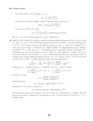
65. 2.9 Modeling with Systems of First-Order DEs
z(t) denote the amounts of substances W, X, Y , and Z, respectively. A model for the radioactive series is
dw
dt
= −λ1w
dx
dt
= λ1w − λ2x
dy
dt
= λ2x − λ3y
dz
dt
= λ3y.
5. The system is
x1 = 2 · 3 +
1
50
x2 −
1
50
x1 · 4 = −
2
25
x1 +
1
50
x2 + 6
x2 =
1
50
x1 · 4 −
1
50
x2 −
1
50
x2 · 3 =
2
25
x1 −
2
25
x2.
6. Let x1, x2, and x3 be the amounts of salt in tanks A, B, and C, respectively, so that
x1 =
1
100
x2 · 2 −
1
100
x1 · 6 =
1
50
x2 −
3
50
x1
x2 =
1
100
x1 · 6 +
1
100
x3 −
1
100
x2 · 2 −
1
100
x2 · 5 =
3
50
x1 −
7
100
x2 +
1
100
x3
x3 =
1
100
x2 · 5 −
1
100
x3 −
1
100
x3 · 4 =
1
20
x2 −
1
20
x3.
7. (a) A model is
dx1
dt
= 3 ·
x2
100 − t
− 2 ·
x1
100 + t
, x1(0) = 100
dx2
dt
= 2 ·
x1
100 + t
− 3 ·
x2
100 − t
, x2(0) = 50.
(b) Since the system is closed, no salt enters or leaves the system and x1(t) + x2(t) = 100 + 50 = 150 for all
time. Thus x1 = 150 − x2 and the second equation in part (a) becomes
dx2
dt
=
2(150 − x2)
100 + t
−
3x2
100 − t
=
300
100 + t
−
2x2
100 + t
−
3x2
100 − t
or
dx2
dt
+
2
100 + t
+
3
100 − t
x2 =
300
100 + t
,
which is linear in x2. An integrating factor is
e2 ln(100+t)−3 ln(100−t)
= (100 + t)2
(100 − t)−3
so
d
dt
[(100 + t)2
(100 − t)−3
x2] = 300(100 + t)(100 − t)−3
.
Using integration by parts, we obtain
(100 + t)2
(100 − t)−3
x2 = 300
1
2
(100 + t)(100 − t)−2
−
1
2
(100 − t)−1
+ c .
Thus
x2 =
300
(100 + t)2
c(100 − t)3
−
1
2
(100 − t)2
+
1
2
(100 + t)(100 − t)
=
300
(100 + t)2
[c(100 − t)3
+ t(100 − t)].
86

66. x
y
t
x,y
50 100
5
10
x
y
t
x,y
10 20
10
5
x
y
t
x,y
10 20
10
5
x
y
t
x,y
10 20
10
5
2.9 Modeling with Systems of First-Order DEs
Using x2(0) = 50 we find c = 5/3000. At t = 30, x2 = (300/1302
)(703
c + 30 · 70) ≈ 47.4 lbs.
8. A model is
dx1
dt
= (4 gal/min)(0 lb/gal) − (4 gal/min)
1
200
x1 lb/gal
dx2
dt
= (4 gal/min)
1
200
x1 lb/gal − (4 gal/min)
1
150
x2 lb/gal
dx3
dt
= (4 gal/min)
1
150
x2 lb/gal − (4 gal/min)
1
100
x3 lb/gal
or
dx1
dt
= −
1
50
x1
dx2
dt
=
1
50
x1 −
2
75
x2
dx3
dt
=
2
75
x2 −
1
25
x3.
Over a long period of time we would expect x1, x2, and x3 to approach 0 because the entering pure water should
flush the salt out of all three tanks.
9. Zooming in on the graph it can be seen that the populations are
first equal at about t = 5.6. The approximate periods of x and y
are both 45.
10. (a) The population y(t) approaches 10,000, while the population x(t)
approaches extinction.
(b) The population x(t) approaches 5,000, while the population y(t)
approaches extinction.
(c) The population y(t) approaches 10,000, while the population x(t)
approaches extinction.
87

67. x
y
t
x,y
10 20
10
5
x
y
t
x,y
20 40
10
5
x
y
t
x,y
20 40
10
5
x
y
t
x,y
20 40
10
5 x
y
t
x,y
20 40
10
5
2.9 Modeling with Systems of First-Order DEs
(d) The population x(t) approaches 5,000, while the population y(t)
approaches extinction.
11. (a) (b)
(c) (d)
In each case the population x(t) approaches 6,000, while the population y(t) approaches 8,000.
12. By Kirchhoff’s first law we have i1 = i2 +i3. By Kirchhoff’s second law, on each loop we have E(t) = Li1 +R1i2
and E(t) = Li1 + R2i3 + q/C so that q = CR1i2 − CR2i3. Then i3 = q = CR1i2 − CR2i3 so that the system is
Li2 + Li3 + R1i2 = E(t)
−R1i2 + R2i3 +
1
C
i3 = 0.
13. By Kirchhoff’s first law we have i1 = i2 + i3. Applying Kirchhoff’s second law to each loop we obtain
E(t) = i1R1 + L1
di2
dt
+ i2R2
and
E(t) = i1R1 + L2
di3
dt
+ i3R3.
Combining the three equations, we obtain the system
L1
di2
dt
+ (R1 + R2)i2 + R1i3 = E
L2
di3
dt
+ R1i2 + (R1 + R3)i3 = E.
14. By Kirchhoff’s first law we have i1 = i2 + i3. By Kirchhoff’s second law, on each loop we have E(t) = Li1 + Ri2
and E(t) = Li1 + q/C so that q = CRi2. Then i3 = q = CRi2 so that system is
Li + Ri2 = E(t)
CRi2 + i2 − i1 = 0.
15. We first note that s(t) + i(t) + r(t) = n. Now the rate of change of the number of susceptible persons, s(t),
is proportional to the number of contacts between the number of people infected and the number who are
88

68. s
i
t
s,i
5 10
5
10
s
i
t
s,i
5 10
5
10
s
i
t
s,i
5 10
5
10
s
i
t
s,i
5 10
5
10
2.9 Modeling with Systems of First-Order DEs
susceptible; that is, ds/dt = −k1si. We use −k1 < 0 because s(t) is decreasing. Next, the rate of change of
the number of persons who have recovered is proportional to the number infected; that is, dr/dt = k2i where
k2 > 0 since r is increasing. Finally, to obtain di/dt we use
d
dt
(s + i + r) =
d
dt
n = 0.
This gives
di
dt
= −
dr
dt
−
ds
dt
= −k2i + k1si.
The system of differential equations is then
ds
dt
= −k1si
di
dt
= −k2i + k1si
dr
dt
= k2i.
A reasonable set of initial conditions is i(0) = i0, the number of infected people at time 0, s(0) = n − i0, and
r(0) = 0.
16. (a) If we know s(t) and i(t) then we can determine r(t) from s + i + r = n.
(b) In this case the system is
ds
dt
= −0.2si
di
dt
= −0.7i + 0.2si.
We also note that when i(0) = i0, s(0) = 10 − i0 since r(0) = 0 and i(t) + s(t) + r(t) = 0 for all values of
t. Now k2/k1 = 0.7/0.2 = 3.5, so we consider initial conditions s(0) = 2, i(0) = 8; s(0) = 3.4, i(0) = 6.6;
s(0) = 7, i(0) = 3; and s(0) = 9, i(0) = 1.
We see that an initial susceptible population greater than k2/k1 results in an epidemic in the sense that
the number of infected persons increases to a maximum before decreasing to 0. On the other hand, when
s(0) < k2/k1, the number of infected persons decreases from the start and there is no epidemic.
89

69. x
y
2.9 Modeling with Systems of First-Order DEs
CHAPTER 2 REVIEW EXERCISES
CHAPTER 2 REVIEW EXERCISES
1. Writing the differential equation in the form y = k(y + A/k) we see that the critical point −A/k is a repeller
for k > 0 and an attractor for k < 0.
2. Separating variables and integrating we have
dy
y
=
4
x
dx
ln y = 4 ln x + c = ln x4
+ c
y = c1x4
.
We see that when x = 0, y = 0, so the initial-value problem has an infinite number of solutions for k = 0 and
no solutions for k = 0.
3.
dy
dx
= (y − 1)2
(y − 3)2
4.
dy
dx
= y(y − 2)2
(y − 4)
5. When n is odd, xn
< 0 for x < 0 and xn
> 0 for x > 0. In this case 0 is unstable. When n is even, xn
> 0 for
x < 0 and for x > 0. In this case 0 is semi-stable.
When n is odd, −xn
> 0 for x < 0 and −xn
< 0 for x > 0. In this case 0 is asymptotically stable. When n is
even, −xn
< 0 for x < 0 and for x > 0. In this case 0 is semi-stable.
6. Using a CAS we find that the zero of f occurs at approximately P = 1.3214. From the graph we observe that
dP/dt > 0 for P < 1.3214 and dP/dt < 0 for P > 1.3214, so P = 1.3214 is an asymptotically stable critical
point. Thus, limt→∞ P(t) = 1.3214.
7.
8. (a) linear in y, homogeneous, exact (b) linear in x
(c) separable, exact, linear in x and y (d) Bernoulli in x
(e) separable (f) separable, linear in x, Bernoulli
(g) linear in x (h) homogeneous
90

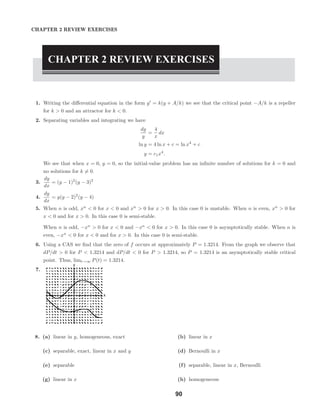
70. CHAPTER 2 REVIEW EXERCISES
(i) Bernoulli (j) homogeneous, exact, Bernoulli
(k) linear in x and y, exact, separable, homoge-
neous
(l) exact, linear in y
(m) homogeneous (n) separable
9. Separating variables and using the identity cos2
x = 1
2 (1 + cos 2x), we have
cos2
x dx =
y
y2 + 1
dy,
1
2
x +
1
4
sin 2x =
1
2
ln y2
+ 1 + c,
and
2x + sin 2x = 2 ln y2
+ 1 + c.
10. Write the differential equation in the form
y ln
x
y
dx = x ln
x
y
− y dy.
This is a homogeneous equation, so let x = uy. Then dx = u dy + y du and the differential equation becomes
y ln u(u dy + y du) = (uy ln u − y) dy or y ln u du = −dy.
Separating variables, we obtain
ln u du = −
dy
y
u ln |u| − u = − ln |y| + c
x
y
ln
x
y
−
x
y
= − ln |y| + c
x(ln x − ln y) − x = −y ln |y| + cy.
11. The differential equation
dy
dx
+
2
6x + 1
y = −
3x2
6x + 1
y−2
is Bernoulli. Using w = y3
, we obtain the linear equation
dw
dx
+
6
6x + 1
w = −
9x2
6x + 1
.
An integrating factor is 6x + 1, so
d
dx
[(6x + 1)w] = −9x2
,
w = −
3x3
6x + 1
+
c
6x + 1
,
and
(6x + 1)y3
= −3x3
+ c.
(Note: The differential equation is also exact.)
12. Write the differential equation in the form (3y2
+ 2x)dx + (4y2
+ 6xy)dy = 0. Letting M = 3y2
+ 2x and
N = 4y2
+ 6xy we see that My = 6y = Nx, so the differential equation is exact. From fx = 3y2
+ 2x we obtain
91

71. CHAPTER 2 REVIEW EXERCISES
f = 3xy2
+ x2
+ h(y). Then fy = 6xy + h (y) = 4y2
+ 6xy and h (y) = 4y2
so h(y) = 4
3 y3
. A one-parameter
family of solutions is
3xy2
+ x2
+
4
3
y3
= c.
13. Write the equation in the form
dQ
dt
+
1
t
Q = t3
ln t.
An integrating factor is eln t
= t, so
d
dt
[tQ] = t4
ln t
tQ = −
1
25
t5
+
1
5
t5
ln t + c
and
Q = −
1
25
t4
+
1
5
t4
ln t +
c
t
.
14. Letting u = 2x + y + 1 we have
du
dx
= 2 +
dy
dx
,
and so the given differential equation is transformed into
u
du
dx
− 2 = 1 or
du
dx
=
2u + 1
u
.
Separating variables and integrating we get
u
2u + 1
du = dx
1
2
−
1
2
1
2u + 1
du = dx
1
2
u −
1
4
ln |2u + 1| = x + c
2u − ln |2u + 1| = 2x + c1.
Resubstituting for u gives the solution
4x + 2y + 2 − ln |4x + 2y + 3| = 2x + c1
or
2x + 2y + 2 − ln |4x + 2y + 3| = c1.
15. Write the equation in the form
dy
dx
+
8x
x2 + 4
y =
2x
x2 + 4
.
An integrating factor is x2
+ 4
4
, so
d
dx
x2
+ 4
4
y = 2x x2
+ 4
3
x2
+ 4
4
y =
1
4
x2
+ 4
4
+ c
and
y =
1
4
+ c x2
+ 4
−4
.
92

72. CHAPTER 2 REVIEW EXERCISES
16. Letting M = 2r2
cos θ sin θ + r cos θ and N = 4r + sin θ − 2r cos2
θ we see that Mr = 4r cos θ sin θ + cos θ = Nθ,
so the differential equation is exact. From fθ = 2r2
cos θ sin θ + r cos θ we obtain f = −r2
cos2
θ + r sin θ + h(r).
Then fr = −2r cos2
θ + sin θ + h (r) = 4r + sin θ − 2r cos2
θ and h (r) = 4r so h(r) = 2r2
. The solution is
−r2
cos2
θ + r sin θ + 2r2
= c.
17. The differential equation has the form (d/dx) [(sin x)y] = 0. Integrating, we have (sin x)y = c or y = c/ sin x.
The initial condition implies c = −2 sin(7π/6) = 1. Thus, y = 1/ sin x, where the interval π < x < 2π is chosen
to include x = 7π/6.
18. Separating variables and integrating we have
dy
y2
= −2(t + 1) dt
−
1
y
= −(t + 1)2
+ c
y =
1
(t + 1)2 + c1
, where −c = c1.
The initial condition y(0) = −1
8 implies c1 = −9, so a solution of the initial-value problem is
y =
1
(t + 1)2 − 9
or y =
1
t2 + 2t − 8
,
where −4 < t < 2.
19. (a) For y < 0,
√
y is not a real number.
(b) Separating variables and integrating we have
dy
√
y
= dx and 2
√
y = x + c.
Letting y(x0) = y0 we get c = 2
√
y0 − x0, so that
2
√
y = x + 2
√
y0 − x0 and y =
1
4
(x + 2
√
y0 − x0)2
.
Since
√
y > 0 for y = 0, we see that dy/dx = 1
2 (x + 2
√
y0 − x0) must be positive. Thus, the interval on
which the solution is defined is (x0 − 2
√
y0, ∞).
20. (a) The differential equation is homogeneous and we let y = ux. Then
(x2
− y2
) dx + xy dy = 0
(x2
− u2
x2
) dx + ux2
(u dx + x du) = 0
dx + ux du = 0
u du = −
dx
x
1
2
u2
= − ln |x| + c
y2
x2
= −2 ln |x| + c1.
The initial condition gives c1 = 2, so an implicit solution is y2
= x2
(2 − 2 ln |x|).
93

73. -2 -1 1 2 x
-2
-1
1
2
y
CHAPTER 2 REVIEW EXERCISES
(b) Solving for y in part (a) and being sure that the initial condition is
still satisfied, we have y = −
√
2 |x|(1 − ln |x|)1/2
, where
−e ≤ x ≤ e so that 1 − ln |x| ≥ 0. The graph of this function indi-
cates that the derivative is not defined at x = 0 and x = e. Thus,
the solution of the initial-value problem is y = −
√
2 x(1 − ln x)1/2
, for
0 < x < e.
21. The graph of y1(x) is the portion of the closed black curve lying in the fourth quadrant. Its interval of definition
is approximately (0.7, 4.3). The graph of y2(x) is the portion of the left-hand black curve lying in the third
quadrant. Its interval of definition is (−∞, 0).
22. The first step of Euler’s method gives y(1.1) ≈ 9 + 0.1(1 + 3) = 9.4. Applying Euler’s method one more time
gives y(1.2) ≈ 9.4 + 0.1(1 + 1.1
√
9.4 ) ≈ 9.8373.
23. From
dP
dt
= 0.018P and P(0) = 4 billion we obtain P = 4e0.018t
so that P(45) = 8.99 billion.
24. Let A = A(t) be the volume of CO2 at time t. From dA/dt = 1.2 − A/4 and A(0) = 16 ft3
we obtain
A = 4.8 + 11.2e−t/4
. Since A(10) = 5.7 ft3
, the concentration is 0.017%. As t → ∞ we have A → 4.8 ft3
or
0.06%.
25. Separating variables, we have
s2 − y2
y
dy = −dx.
Substituting y = s sin θ, this becomes
s2 − s2 sin2
θ
s sin θ
(s cos θ)dθ = −dx
s
cos2
sin θ
dθ = − dx
s
1 − sin2
θ
sin θ
dθ = −x + c
s (csc θ − sin θ)dθ = −x + c
s ln | csc θ − cot θ| + s cos θ = −x + c
s ln
s
y
−
s2 − y2
y
+ s
s2 − y2
s
= −x + c.
Letting s = 10, this is
10 ln
10
y
−
100 − y2
y
+ 100 − y2 = −x + c.
Letting x = 0 and y = 10 we determine that c = 0, so the solution is
10 ln
10
y
−
100 − y2
y
+ 100 − y2 = −x.
26. From V dC/dt = kA(Cs − C) and C(0) = C0 we obtain C = Cs + (C0 − Cs)e−kAt/V
.
94

74. CHAPTER 2 REVIEW EXERCISES
27. (a) The differential equation
dT
dt
= k(T − Tm) = k[T − T2 − B(T1 − T)]
= k[(1 + B)T − (BT1 + T2)] = k(1 + B) T −
BT1 + T2
1 + B
is autonomous and has the single critical point (BT1 + T2)/(1 + B). Since k < 0 and B > 0, by phase-line
analysis it is found that the critical point is an attractor and
lim
t→∞
T(t) =
BT1 + T2
1 + B
.
Moreover,
lim
t→∞
Tm(t) = lim
t→∞
[T2 + B(T1 − T)] = T2 + B T1 −
BT1 + T2
1 + B
=
BT1 + T2
1 + B
.
(b) The differential equation is
dT
dt
= k(T − Tm) = k(T − T2 − BT1 + BT)
or
dT
dt
− k(1 + B)T = −k(BT1 + T2).
This is linear and has integrating factor e− k(1+B)dt
= e−k(1+B)t
. Thus,
d
dt
[e−k(1+B)t
T] = −k(BT1 + T2)e−k(1+B)t
e−k(1+B)t
T =
BT1 + T2
1 + B
e−k(1+B)t
+ c
T(t) =
BT1 + T2
1 + B
+ cek(1+B)t
.
Since k is negative, limt→∞ T(t) = (BT1 + T2)/(1 + B).
(c) The temperature T(t) decreases to (BT1 + T2)/(1 + B), whereas Tm(t) increases to (BT1 + T2)/(1 + B) as
t → ∞. Thus, the temperature (BT1 + T2)/(1 + B), (which is a weighted average,
B
1 + B
T1 +
1
1 + B
T2,
of the two initial temperatures), can be interpreted as an equilibrium temperature. The body cannot get
cooler than this value whereas the medium cannot get hotter than this value.
28. (a) By separation of variables and partial fractions,
ln
T − Tm
T + Tm
− 2 tan−1 T
Tm
= 4T3
mkt + c.
Then rewrite the right-hand side of the differential equation as
dT
dt
= k(T4
− T4
m) = [(Tm + (T − Tm))4
− T4
m]
= kT4
m 1 +
T − Tm
Tm
4
− 1
= kT4
m 1 + 4
T − Tm
Tm
+ 6
T − Tm
Tm
2
· · · − 1 ← binomial expansion
95

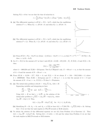
75. 10 20
10
20
time
seconds
height
inches
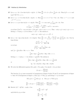
0 24.0000
1 22.0520
2 20.1864
3 18.4033
4 16.7026
5 15.0844
6 13.5485
7 12.0952
8 10.7242
9 9.4357
10 8.2297
11 7.1060
12 6.0648
CHAPTER 2 REVIEW EXERCISES
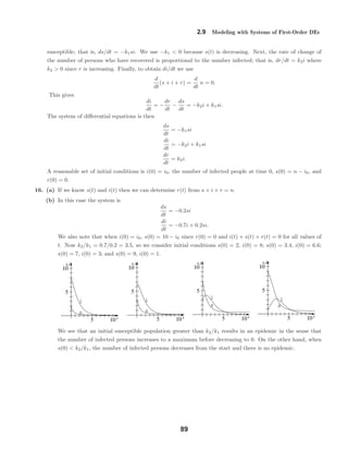
(b) When T − Tm is small compared to Tm, every term in the expansion after the first two can be ignored,
giving
dT
dt
≈ k1(T − Tm), where k1 = 4kT3
m.
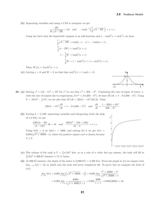
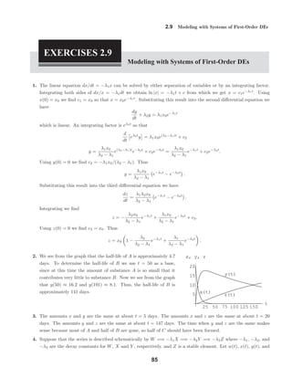
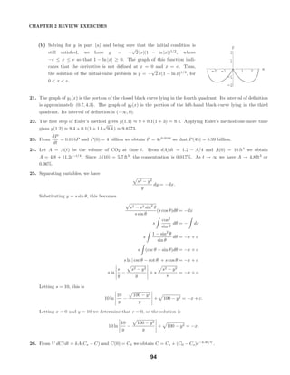
29. We first solve (1 − t/10)di/dt + 0.2i = 4. Separating variables we obtain di/(40 − 2i) =
dt/(10 − t). Then
−
1
2
ln |40 − 2i| = − ln |10 − t| + c or
√
40 − 2i = c1(10 − t).
Since i(0) = 0 we must have c1 = 2/
√
10 . Solving for i we get i(t) = 4t − 1
5 t2
, 0 ≤ t < 10.
For t ≥ 10 the equation for the current becomes 0.2i = 4 or i = 20. Thus
i(t) =
4t − 1
5 t2
, 0 ≤ t < 10
20, t ≥ 10.
The graph of i(t) is given in the figure.
30. From y 1 + (y )2
= k we obtain dx = (
√
y/
√
k − y )dy. If y = k sin2
θ then
dy = 2k sin θ cos θ dθ, dx = 2k
1
2
−
1
2
cos 2θ dθ, and x = kθ −
k
2
sin 2θ + c.
If x = 0 when θ = 0 then c = 0.
31. Letting c = 0.6, Ah = π( 1
32 · 1
12 )2
, Aw = π · 12
= π, and g = 32, the differential equation becomes
dh/dt = −0.00003255
√
h . Separating variables and integrating, we get 2
√
h = −0.00003255t + c, so h =
(c1 − 0.00001628t)2
. Setting h(0) = 2, we find c =
√
2 , so h(t) = (
√
2 − 0.00001628t)2
, where h is measured in
feet and t in seconds.
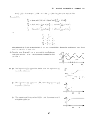
32. One hour is 3,600 seconds, so the hour mark should be placed at
h(3600) = [
√
2 − 0.00001628(3600)]2
≈ 1.838 ft ≈ 22.0525 in.
up from the bottom of the tank. The remaining marks corresponding to the passage
of 2, 3, 4, . . . , 12 hours are placed at the values shown in the table. The marks are
not evenly spaced because the water is not draining out at a uniform rate; that is,
h(t) is not a linear function of time.
33. In this case Aw = πh2
/4 and the differential equation is
dh
dt
= −
1
7680
h−3/2
.
Separating variables and integrating, we have
h3/2
dh = −
1
7680
dt
2
5
h5/2
= −
1
7680
t + c1.
96

76. r
h
−1 1
1
2
CHAPTER 2 REVIEW EXERCISES
Setting h(0) = 2 we find c1 = 8
√
2/5, so that
2
5
h5/2
= −
1
7680
t +
8
√
2
5
,
h5/2
= 4
√
2 −
1
3072
t,
and
h = 4
√
2 −
1
3072
t
2/5
.
In this case h(4 hr) = h(14,400 s) = 11.8515 inches and h(5 hr) = h(18,000 s) is not a real number. Using a
CAS to solve h(t) = 0, we see that the tank runs dry at t ≈ 17,378 s ≈ 4.83 hr. Thus, this particular conical
water clock can only measure time intervals of less than 4.83 hours.
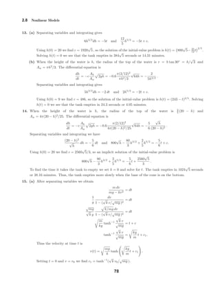
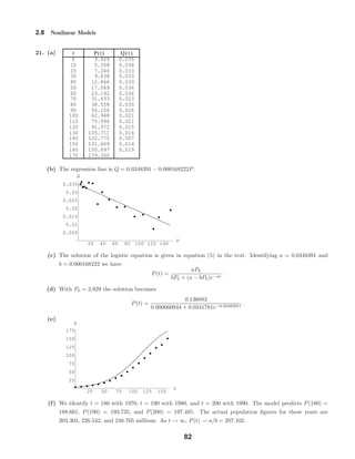
34. If we let rh denote the radius of the hole and Aw = π[f(h)]2
, then the
differential equation dh/dt = −k
√
h, where k = cAh
√
2g/Aw, becomes
dh
dt
= −
cπr2
h
√
2g
π[f(h)]2
√
h = −
8cr2
h
√
h
[f(h)]2
.
For the time marks to be equally spaced, the rate of change of the height must be
a constant; that is, dh/dt = −a. (The constant is negative because the height is
decreasing.) Thus
−a = −
8cr2
h
√
h
[f(h)]2
, [f(h)]2
=
8cr2
h
√
h
a
, and r = f(h) = 2rh
2c
a
h1/4
.
Solving for h, we have
h =
a2
64c2r4
h
r4
.
The shape of the tank with c = 0.6, a = 2 ft/12 hr = 1 ft/21,600 s, and rh = 1/32(12) = 1/384 is shown in the
above figure.
35. From dx/dt = k1x(α − x) we obtain
1/α
x
+
1/α
α − x
dx = k1 dt
so that x = αc1eαk1t
/(1 + c1eαk1t
). From dy/dt = k2xy we obtain
ln |y| =
k2
k1
ln 1 + c1eαk1t
+ c or y = c2 1 + c1eαk1t k2/k1
.
36. In tank A the salt input is
7
gal
min
2
lb
gal
+ 1
gal
min
x2
100
lb
gal
= 14 +
1
100
x2
lb
min
.
The salt output is
3
gal
min
x1
100
lb
gal
+ 5
gal
min
x1
100
lb
gal
=
2
25
x1
lb
min
.
In tank B the salt input is
5
gal
min
x1
100
lb
gal
=
1
20
x1
lb
min
.
The salt output is
1
gal
min
x2
100
lb
gal
+ 4
gal
min
x2
100
lb
gal
=
1
20
x2
lb
min
.
97

77. x
y
-5 5
-5
5
CHAPTER 2 REVIEW EXERCISES
The system of differential equations is then
dx1
dt
= 14 +
1
100
x2 −
2
25
x1
dx2
dt
=
1
20
x1 −
1
20
x2.
37. From y = −x − 1 + c1ex
we obtain y = y + x so that the differential equation of the orthogonal family is
dy
dx
= −
1
y + x
or
dx
dy
+ x = −y.
This is a linear differential equation and has integrating factor e dy
= ey
, so
d
dy
[ey
x] = −yey
ey
x = −yey
+ ey
+ c2
x = −y + 1 + c2e−y
.
38. Differentiating the family of curves, we have
y = −
1
(x + c1)2
= −
1
y2
.
The differential equation for the family of orthogonal trajectories is then
y = y2
. Separating variables and integrating we get
dy
y2
= dx
−
1
y
= x + c1
y = −
1
x + c1
.
98