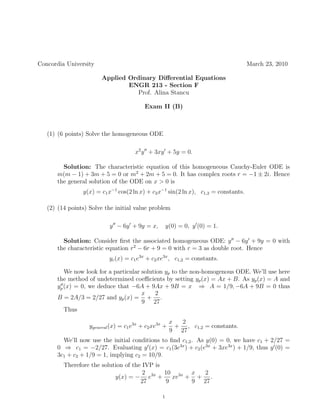
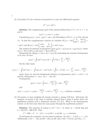
1) The document contains an exam with 4 problems related to ordinary differential equations. 2) The first problem involves solving a homogeneous Cauchy-Euler differential equation. 3) The second problem involves using an initial value problem to find the general solution of a non-homogeneous differential equation, then applying initial conditions to determine constants. 4) The third problem uses the method of variation of parameters to solve a non-homogeneous differential equation. 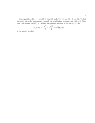5) The fourth problem applies an equation of motion to a physical system of a mass on a spring to determine the instantaneous velocity when the mass passes through equilibrium.

1. Concordia University March 23, 2010
Applied Ordinary Differential Equations
ENGR 213 - Section F
Prof. Alina Stancu
Exam II (B)
(1) (6 points) Solve the homogeneous ODE
x2 y + 3xy + 5y = 0.
Solution: The characteristic equation of this homogeneous Cauchy-Euler ODE is
m(m − 1) + 3m + 5 = 0 or m2 + 2m + 5 = 0. It has complex roots r = −1 ± 2i. Hence
the general solution of the ODE on x > 0 is
y(x) = c1 x−1 cos(2 ln x) + c2 x−1 sin(2 ln x), c1,2 = constants.
(2) (14 points) Solve the initial value problem
y − 6y + 9y = x, y(0) = 0, y (0) = 1.
Solution: Consider first the associated homogeneous ODE: y − 6y + 9y = 0 with
the characteristic equation r2 − 6r + 9 = 0 with r = 3 as double root. Hence
yc (x) = c1 e3x + c2 xe3x , c1,2 = constants.
We now look for a particular solution yp to the non-homogenous ODE. We’ll use here
the method of undetermined coefficients by setting yp (x) = Ax + B. As yp (x) = A and
yp (x) = 0, we deduce that −6A + 9Ax + 9B = x ⇒ A = 1/9, −6A + 9B = 0 thus
x 2
B = 2A/3 = 2/27 and yp (x) = + .
9 27
Thus
x 2
ygeneral (x) = c1 e3x + c2 xe3x + + , c1,2 = constants.
9 27
We’ll now use the initial conditions to find c1,2 . As y(0) = 0, we have c1 + 2/27 =
0 ⇒ c1 = −2/27. Evaluating y (x) = c1 (3e3x ) + c2 (e3x + 3xe3x ) + 1/9, thus y (0) =
3c1 + c2 + 1/9 = 1, implying c2 = 10/9.
Therefore the solution of the IVP is
2 10 3x x 2
y(x) = − e3x + xe + + .
27 9 9 27
1

2. 2
(3) (10 points) Use the variation of parameters to solve the differential equation
y + y = sin2 x.
Solution: The complementary part of the solution follows from r2 +1 = 0 ⇒ r = ±i
and is
yc (x) = c1 cos x + c2 sin x.
Considering y1 (x) = cos x, y2 (x) = sin x, the Wronskian is W (x) = 1 = 0 for all real
0 sin x
x’s. To find the complementary solution we calculate W1 (x) = det 2 =
sin x cos x
cos x 0
− sin3 x and W2 (x) = det = sin2 x cos x.
− sin x sin2 x
The method of variation of parameters gives yp (x) = y1 (x)u1 (x) + y2 (x)u2 (x), where
u1 (x) = W1 (x)/W (x) and u2 (x) = W2 (x)/W (x).
Integrating (by taking u = sin x du = cos x dx) and taking the constant of integration
to be zero, we have
u3 sin3 x
u2 (x) = (sin2 x cos x) dx = u2 du = = .
3 3
On the other hand,
u3 cos3 x
u1 (x) = − sin3 x dx = − sin x (1 − cos2 x) dx = (1 − u2 ) du = u − = cos x − ,
3 3
where above we used the fundamental identity of trigonometry (sin2 x + cos2 x = 1)
and the substitution u = cos x, du = − sin x dx.
Consequently,
cos3 x sin3 x
yp (x) = cos x · cos x − + sin x ·
3 3
and
cos4 x sin4 x
y(x) = c1 cos x + c2 sin x − + cos2 x + , c1,2 = arbitrary constants.
3 3
(4) (10 points) A mass weighing 64 pounds stretches a spring 0.32 foot. Determine the
equation of motion if the mass is initially released from a point 6 inches above the
equilibrium position with a downward velocity of 5 ft/s. What is the instantaneous
velocity at the first time when the mass passes through the equilibrium position?
Solution: The equation of motion is mx + kx = 0, where m = 64/32 slug and
k = 64/0.32 = 200 ft/lb. Thus
x + 100x = 0 ⇒ x(t) = c1 cos 10t + c2 sin 10t, c1,2 = constants.
To determine the constants, use the initial conditions. As x(0) = −1/2 ft, c1 = −1/2.
Additionally, x (t) = −10c1 sin 10t + 10c2 cos 10t, thus x (0) = 5 ft/sec and 10c2 = 5.

3. 3
Consequently, x(t) = − 1 cos 10t + 1 sin 10t and x (t) = 5 sin 10t + 5 cos 10t. To find
2 2
the time when the mass passes through the equilibrium position, set x(t) = 0. Note
that this implies tan(10t) = 1 whose first positive solution is for 10t = π/4. So
√ √
2 2 √
x (π/40) = 5 +5 = 5 2 ft/sec
2 2
is the answer needed.