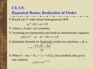
The document discusses solving second order linear homogeneous ordinary differential equations (ODEs) with repeated real roots. It presents the general solution in this case as the sum of two terms: the complementary function, which is the product of an exponential term and a multiplying factor v(t); and the particular integral. Finding the multiplying factor v(t) involves substituting the known solution into the ODE and reducing to a first order equation to solve for v'. The method of reduction of order is also introduced to find the second solution for ODEs with non-constant coefficients, by assuming the second solution is the product of the known first solution and an unknown function v(t). Examples demonstrate finding the general solution using both repeated roots

1. Ch 3.5:
Repeated Roots; Reduction of Order
Recall our 2nd
order linear homogeneous ODE
where a, b and c are constants.
Assuming an exponential soln leads to characteristic equation:
Quadratic formula (or factoring) yields two solutions, r1 & r2:
When b2
– 4ac = 0, r1 = r2 = -b/2a, since method only gives
one solution:
0=+′+′′ cyybya
0)( 2
=++⇒= cbrarety rt
a
acbb
r
2
42
−±−
=
atb
cety 2/
1 )( −
=

2. Second Solution: Multiplying Factor v(t)
We know that
Since y1 and y2 are linearly dependent, we generalize this
approach and multiply by a function v, and determine
conditions for which y2 is a solution:
Then
solutiona)()(solutiona)( 121 tcytyty =⇒
atbatb
etvtyety 2/
2
2/
1 )()(trysolutiona)( −−
=⇒=
atbatbatbatb
atbatb
atb
etv
a
b
etv
a
b
etv
a
b
etvty
etv
a
b
etvty
etvty
2/
2
2
2/2/2/
2
2/2/
2
2/
2
)(
4
)(
2
)(
2
)()(
)(
2
)()(
)()(
−−−−
−−
−
+′−′−′′=′′
−′=′
=

3. Finding Multiplying Factor v(t)
Substituting derivatives into ODE, we seek a formula for v:
0=+′+′′ cyybya
43
2
222
22
22
2
2
2/
)(0)(
0)(
4
4
)(
0)(
4
4
4
)(0)(
4
4
4
2
4
)(
0)(
24
)(
0)()(
2
)()(
4
)()(
0)()(
2
)()(
4
)()(
ktktvtv
tv
a
acb
tva
tv
a
ac
a
b
tvatv
a
ac
a
b
a
b
tva
tvc
a
b
a
b
tva
tcvtv
a
b
tvbtv
a
b
tvbtva
tcvtv
a
b
tvbtv
a
b
tv
a
b
tvae atb
+=⇒=′′
=




 −
−′′
=





+
−
+′′⇔=





+−+′′
=





+−+′′
=+−′++′−′′
=






+



−′+





+′−′′−

4. General Solution
To find our general solution, we have:
Thus the general solution for repeated roots is
( )
abtabt
abtabt
abtabt
tecec
ektkek
etvkekty
2/
2
2/
1
2/
43
2/
1
2/
2
2/
1 )()(
−−
−−
−−
+=
++=
+=
abtabt
tececty 2/
2
2/
1)( −−
+=

5. Wronskian
The general solution is
Thus every solution is a linear combination of
The Wronskian of the two solutions is
Thus y1and y2 form a fundamental solution set for equation.
abtabt
tececty 2/
2
2/
1)( −−
+=
abtabt
tetyety 2/
2
2/
1 )(,)( −−
==
te
a
bt
e
a
bt
e
e
a
bt
e
a
b
tee
tyyW
abt
abtabt
abtabt
abtabt
allfor0
22
1
2
1
2
))(,(
/
//
2/2/
2/2/
21
≠=






+





−=






−−
=
−
−−
−−
−−

6. Example 1
Consider the initial value problem
Assuming exponential soln leads to characteristic equation:
Thus the general solution is
Using the initial conditions:
Thus
( ) ( ) 10,10,02 =′==+′+′′ yyyyy
10)1(012)( 22
−=⇔=+⇔=++⇒= rrrrety rt
tt
tececty −−
+= 21)(
2,1
1
1
21
21
1
==⇒



=+−
=
cc
cc
c
tt
teety −−
+= 2)(

7. Example 2
Consider the initial value problem
Assuming exponential soln leads to characteristic equation:
Thus the general solution is
Using the initial conditions:
Thus
( ) ( ) 2/10,20,025.0 =′==+′−′′ yyyyy
2/10)2/1(025.0)( 22
=⇔=−⇔=+−⇒= rrrrety rt
2/
2
2/
1)( tt
tececty +=
2
1
,2
2
1
2
1
2
21
21
1
−==⇒




=+
=
cc
cc
c
2/2/
2
1
2)( tt
teety −=

8. Example 3
Consider the initial value problem
Assuming exponential soln leads to characteristic equation:
Thus the general solution is
Using the initial conditions:
Thus
( ) ( ) 2/30,20,025.0 =′==+′−′′ yyyyy
2/10)2/1(025.0)( 22
=⇔=−⇔=+−⇒= rrrrety rt
2/
2
2/
1)( tt
tececty +=
2
1
,2
2
3
2
1
2
21
21
1
==⇒




=+
=
cc
cc
c
2/2/
2
1
2)( tt
teety +=

9. Reduction of Order
The method used so far in this section also works for
equations with nonconstant coefficients:
That is, given that y1 is solution, try y2 = v(t)y1:
Substituting these into ODE and collecting terms,
Since y1 is a solution to the differential equation, this last
equation reduces to a first order equation in v′ :
0)()( =+′+′′ ytqytpy
)()()()(2)()()(
)()()()()(
)()()(
1112
112
12
tytvtytvtytvty
tytvtytvty
tytvty
′′+′′+′′=′′
′+′=′
=
( ) ( ) 02 111111 =+′+′′+′+′+′′ vqyypyvpyyvy
( ) 02 111 =′+′+′′ vpyyvy

10. Example 4: Reduction of Order (1 of 3)
Given the variable coefficient equation and solution y1,
use reduction of order method to find a second solution:
Substituting these into ODE and collecting terms,
,)(;0,03 1
1
2 −
=>=+′+′′ ttytyytyt
321
2
21
2
1
2
)(2)(2)()(
)()()(
)()(
−−−
−−
−
+′−′′=′′
−′=′
=
ttvttvttvty
ttvttvty
ttvty
( ) ( )
)()(where,0
0
03322
0322
111
1213212
tvtuuut
vvt
vtvtvvtvtv
vtvttvtvttvtvt
′==+′⇔
=′+′′⇔
=+−′++′−′′⇔
=+−′++′−′′
−−−
−−−−−−

11. Example 4: Finding v(t) (2 of 3)
To solve
for u, we can use the separation of variables method:
Thus
and hence
.0since,
lnln
1
0
11
>=⇔=⇔
+−=⇔−=⇔=+
−−
∫∫
tctuetu
Ctudt
tu
du
u
dt
du
t
C
)()(,0 tvtuuut ′==+′
t
c
v =′
ktctv += ln)(

12. Example 4: General Solution (3 of 3)
We have
Thus
Recall
and hence we can neglect the second term of y2 to obtain
Hence the general solution to the differential equation is
( ) 111
2 lnln)( −−−
+=+= tktcttktcty
ktctv += ln)(
.ln)( 1
2 ttty −
=
1
1 )( −
= tty
ttctcty ln)( 1
2
1
1
−−
+=