Downloaded 238 times
![Calibration Curve Procedure
1. Prepare a series of standard solutions
(analyte solutions with known
concentrations).
2. Plot [analyte] vs. Analytical Signal.
3. Use signal for unknown to find [analyte].](https://image.slidesharecdn.com/calibration-141112131942-conversion-gate02/75/Calibration-3-2048.jpg)
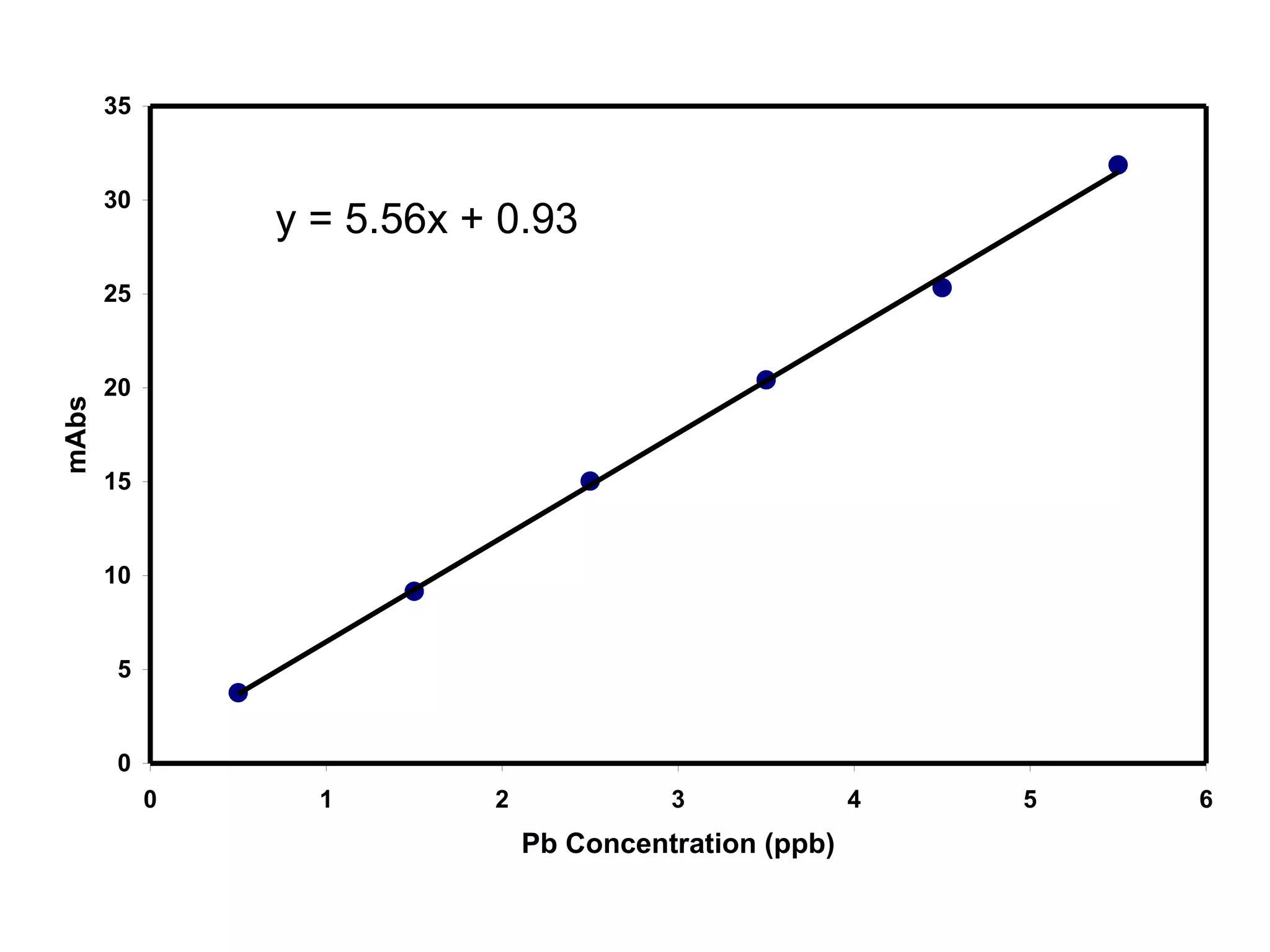
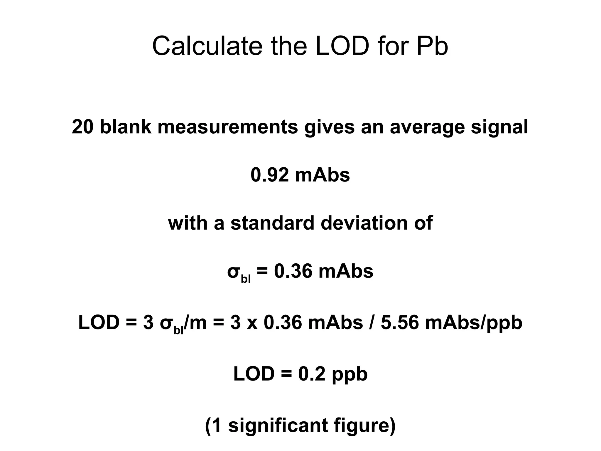
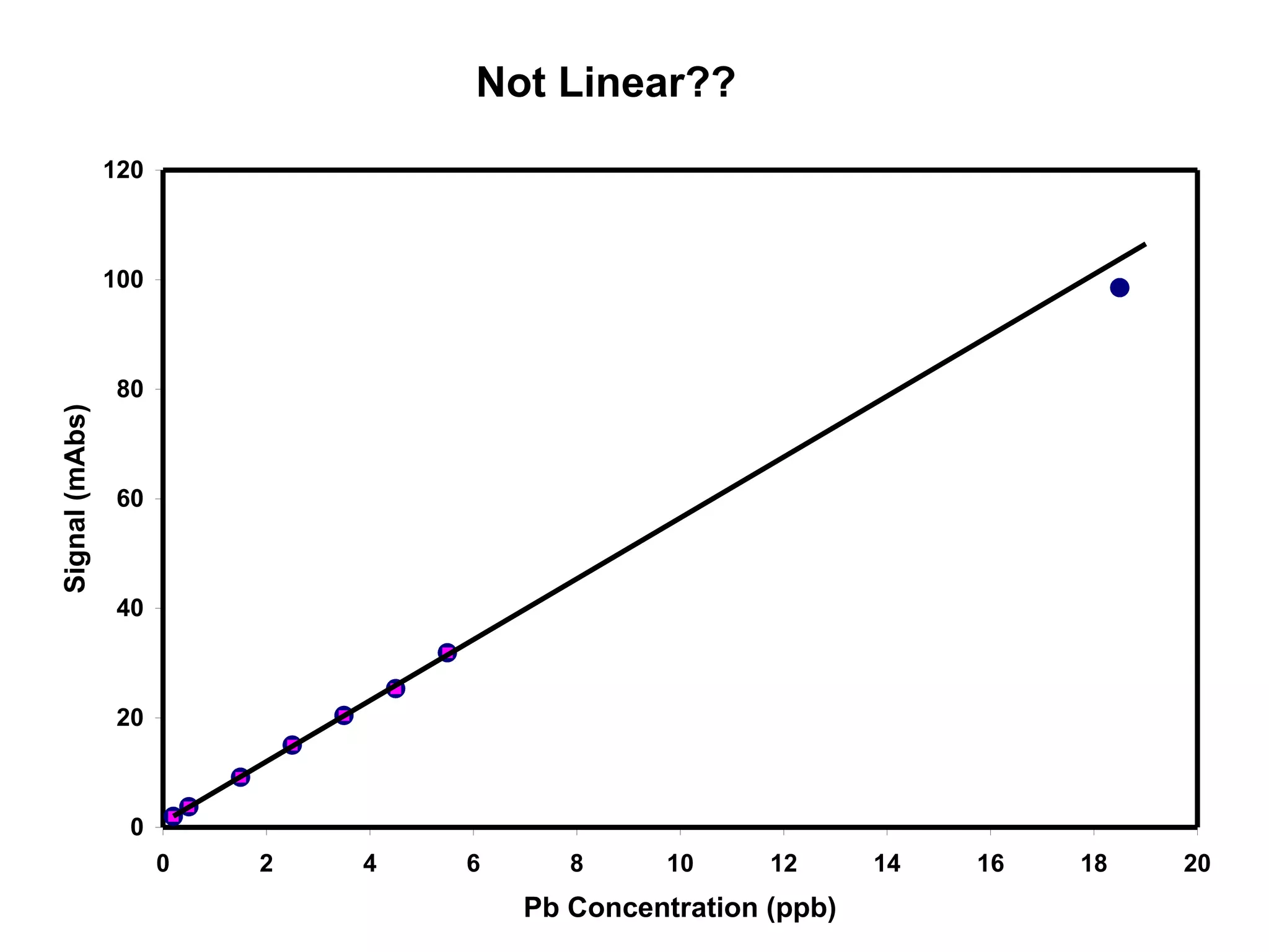
![Example: Pb in Blood by GFAAS
[Pb] Signal
(ppb) (mAbs)
0.50 3.76
1.50 9.16
2.50 15.03
3.50 20.42
4.50 25.33
5.50 31.87
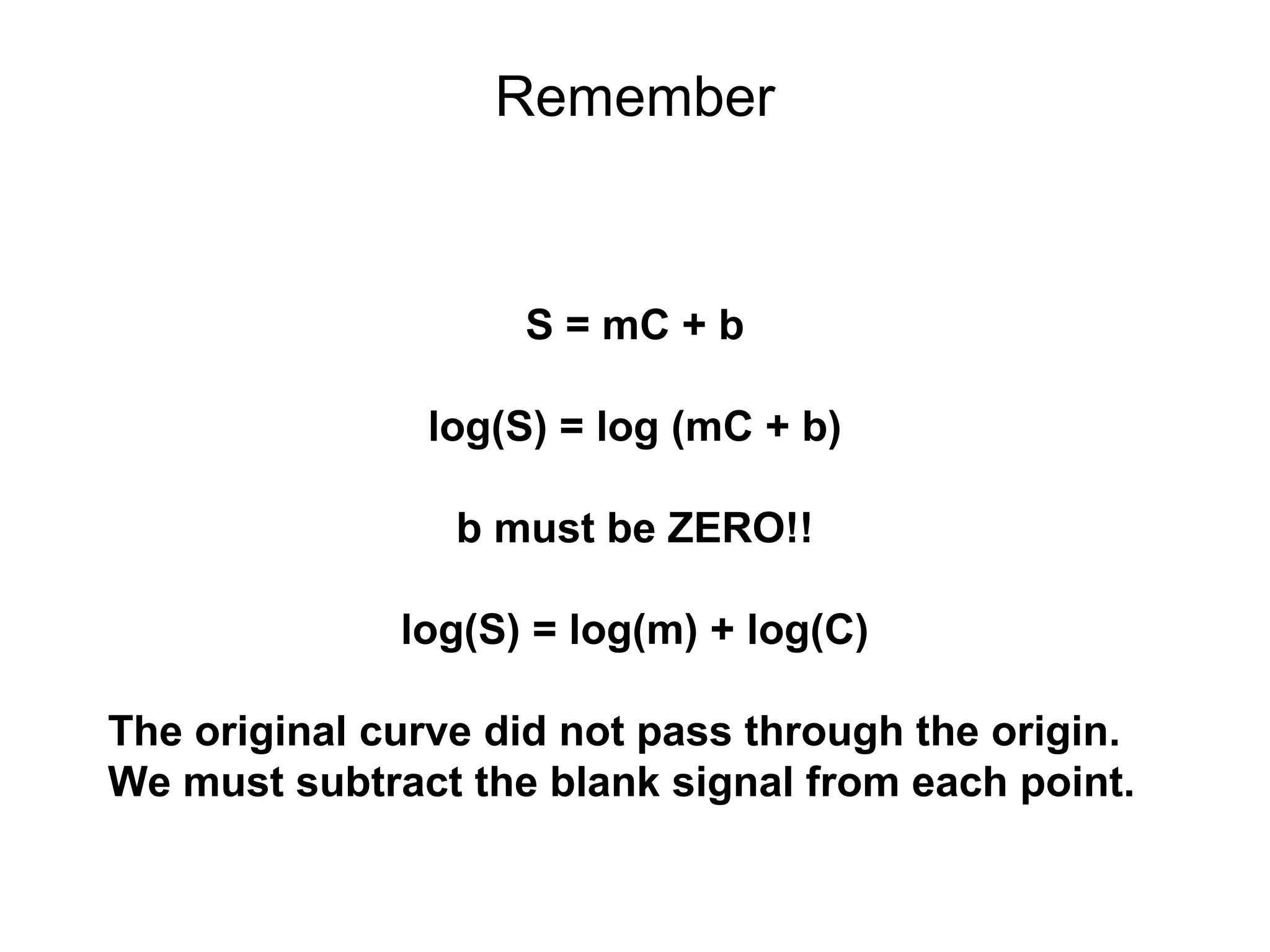
Results of linear regression:
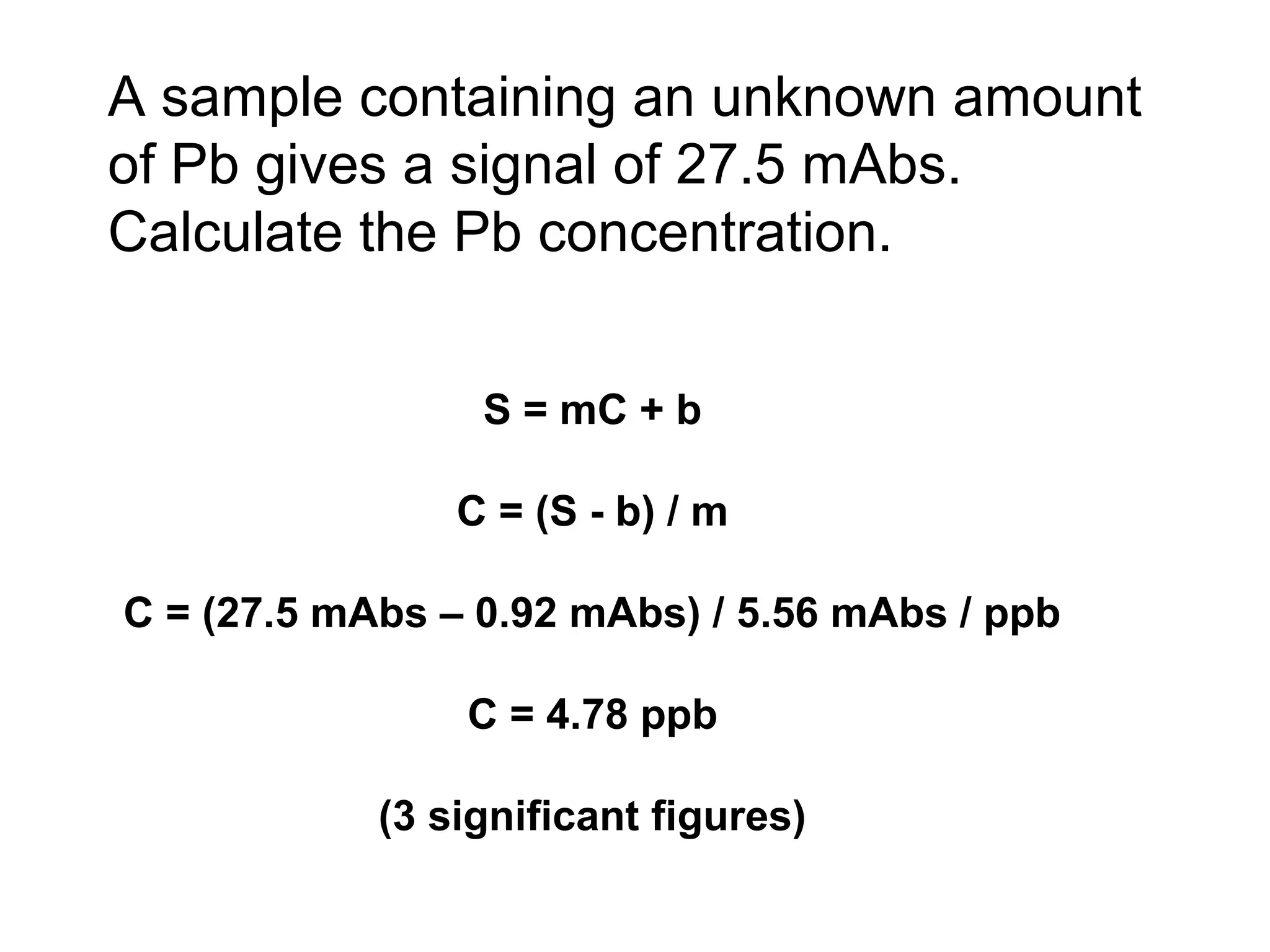
S = mC + b
m = 5.56 mAbs/ppb
b = 0.93 mAbs](https://image.slidesharecdn.com/calibration-141112131942-conversion-gate02/75/Calibration-4-2048.jpg)
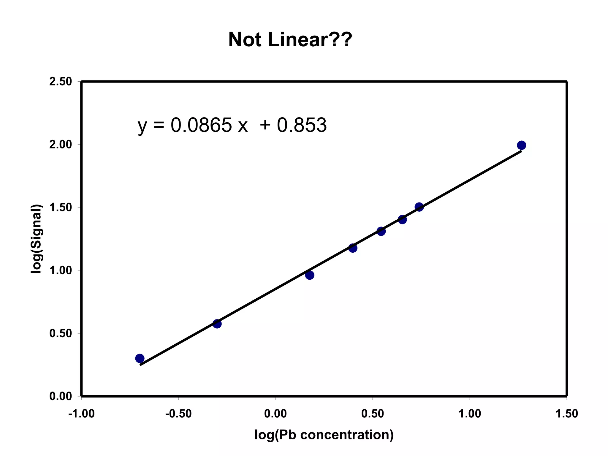
![Find the Linearity
Calculate the slope of the log-log plot
log[Pb] log(S)
-0.70 0.30
-0.30 0.58
0.18 0.96
0.40 1.18
0.54 1.31
0.65 1.40
0.74 1.50
1.27 1.99](https://image.slidesharecdn.com/calibration-141112131942-conversion-gate02/75/Calibration-11-2048.jpg)
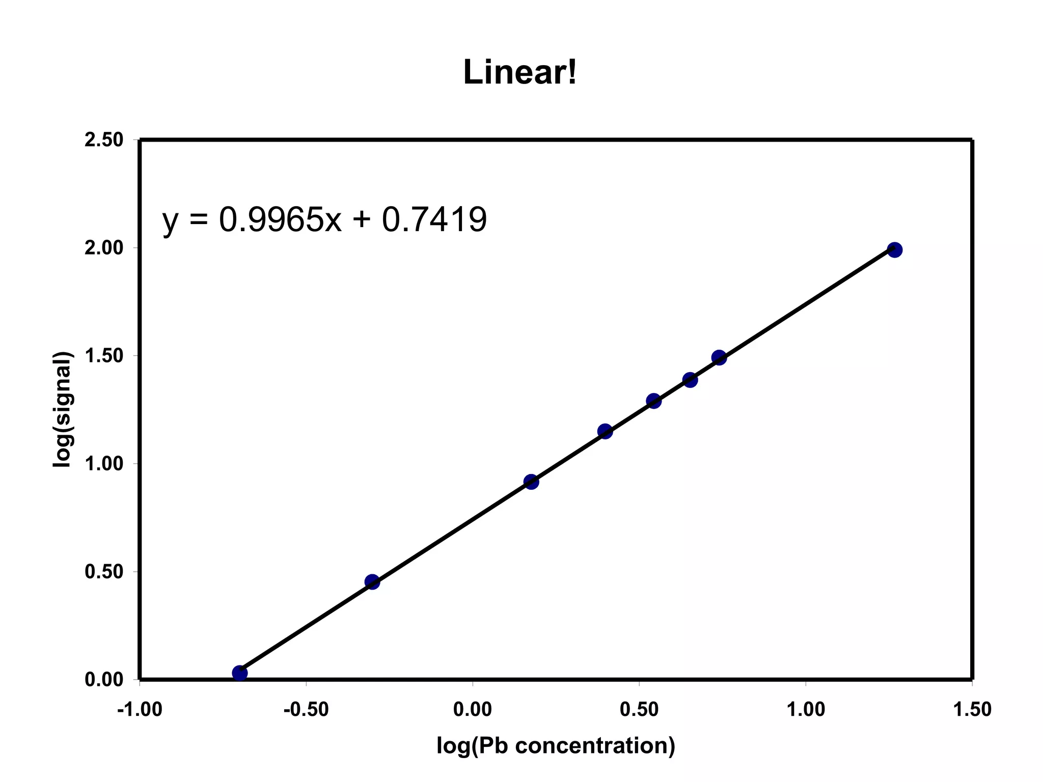
![Corrected Data
[Pb] Signal
(ppb) (mAbs)
0.20 1.07
0.50 2.83
1.50 8.23
2.50 14.10
3.50 19.49
4.50 24.40
5.50 30.94
18.50 97.59
log[Pb] log(S)
-0.70 0.03
-0.30 0.45
0.18 0.92
0.40 1.15
0.54 1.29
0.65 1.39
0.74 1.49
1.27 1.99](https://image.slidesharecdn.com/calibration-141112131942-conversion-gate02/75/Calibration-15-2048.jpg)
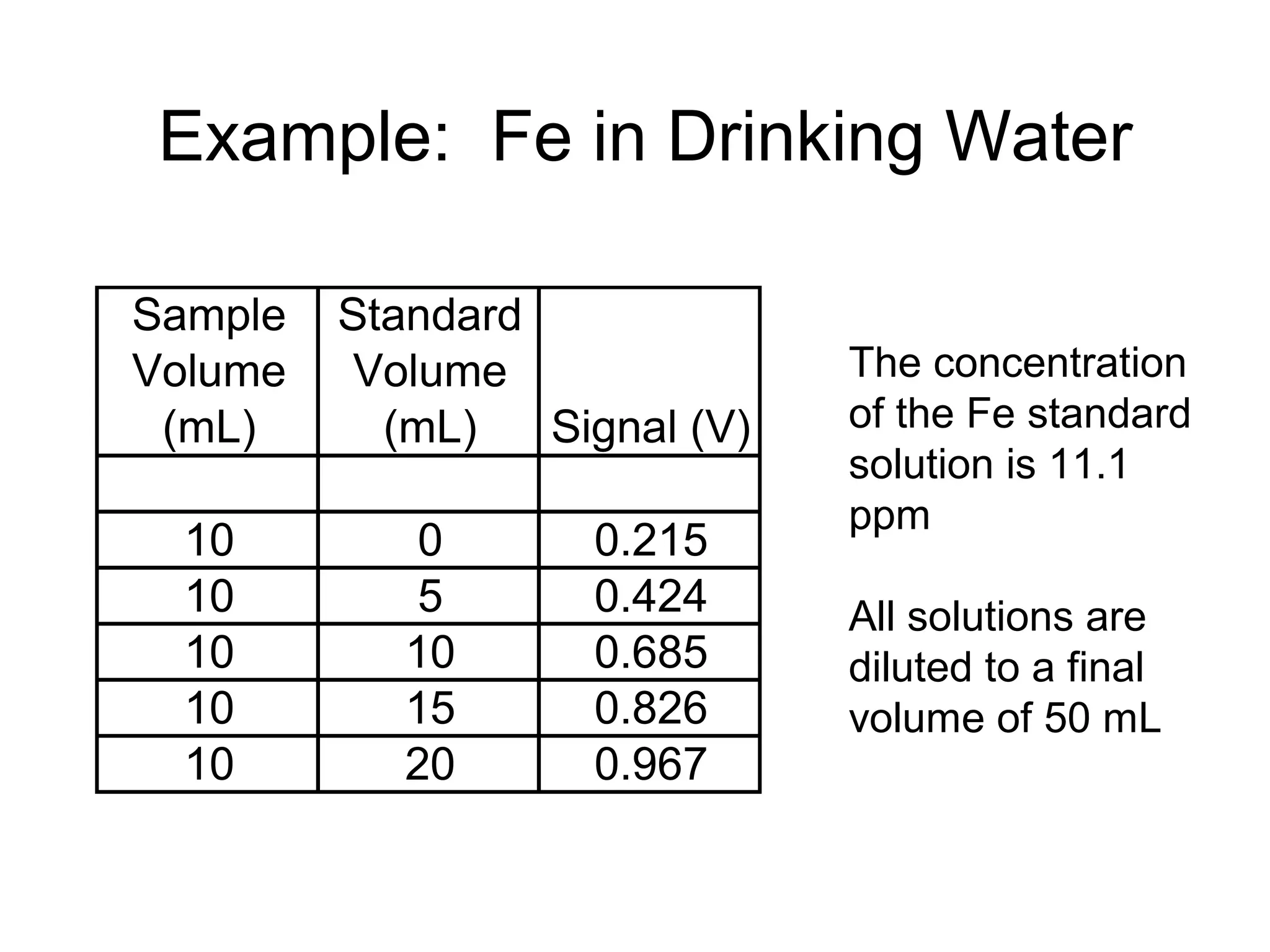
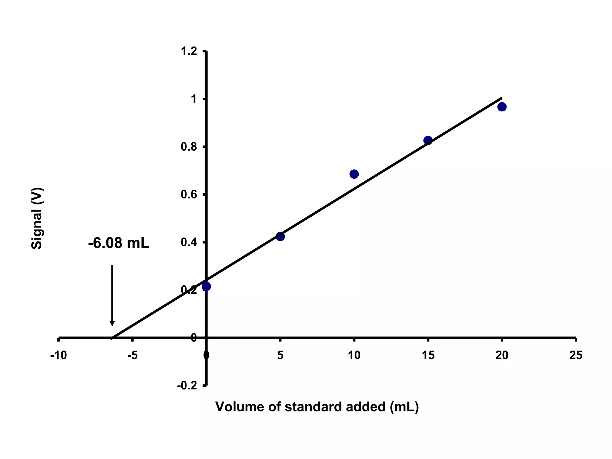
![[Fe] = ?
x-intercept = -6.08 mL
Therefore, 10 mL of sample diluted to 50 mL would
give a signal equivalent to 6.08 mL of standard
diluted to 50 mL.
Vsam x [Fe]sam = Vstd x [Fe]std
10.0 mL x [Fe] = 6.08 mL x 11.1 ppm
[Fe] = 6.75 ppm](https://image.slidesharecdn.com/calibration-141112131942-conversion-gate02/75/Calibration-22-2048.jpg)
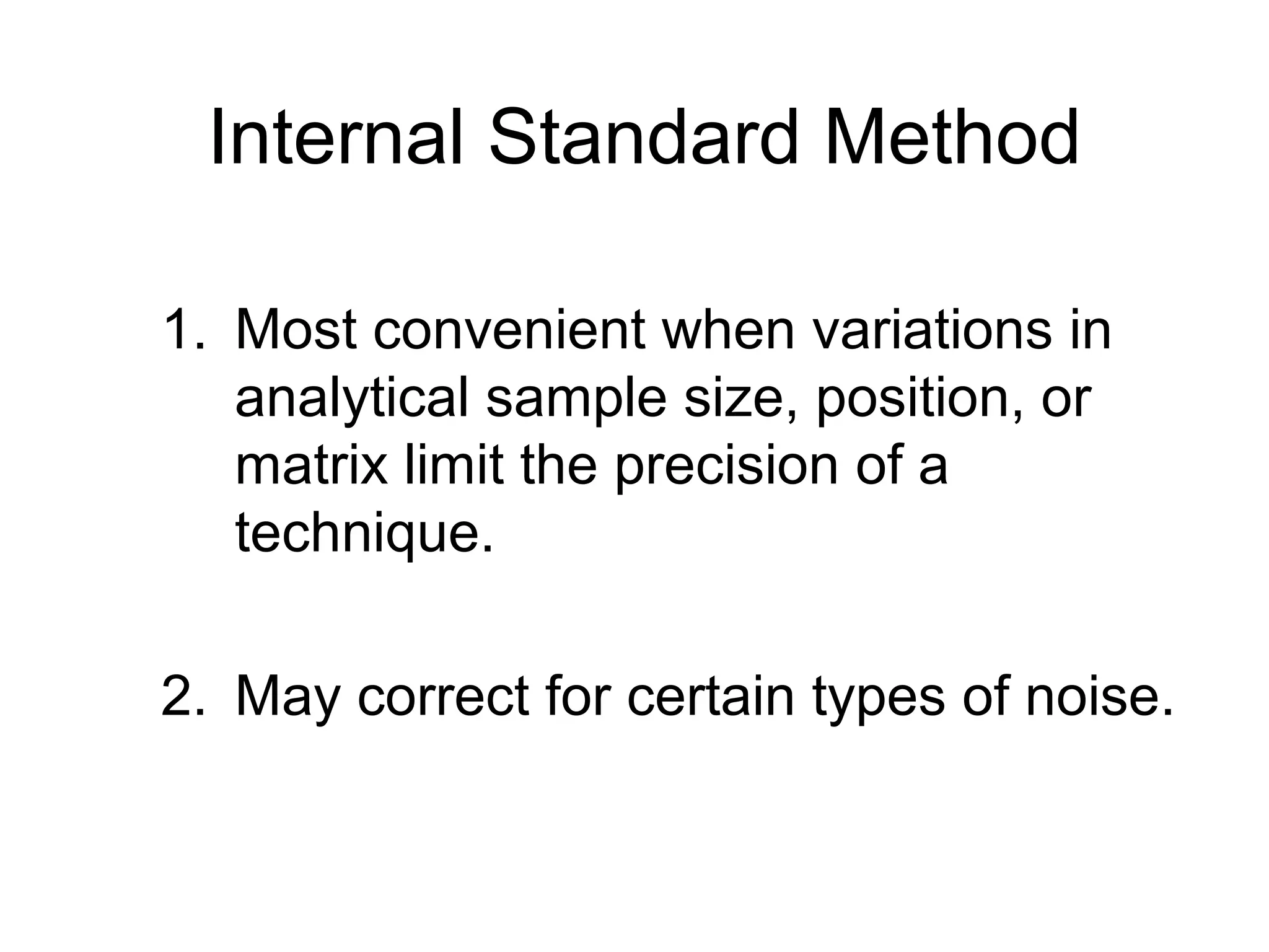
![Internal Standard Procedure
1. Prepare a set of standard solutions for
analyte (A) as with the calibration curve
method, but add a constant amount of a
second species (B) to each solution.
2. Prepare a plot of SA/SB versus [A].](https://image.slidesharecdn.com/calibration-141112131942-conversion-gate02/75/Calibration-24-2048.jpg)
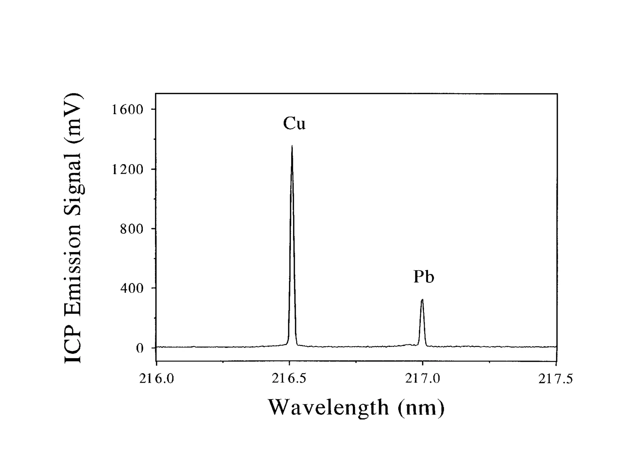
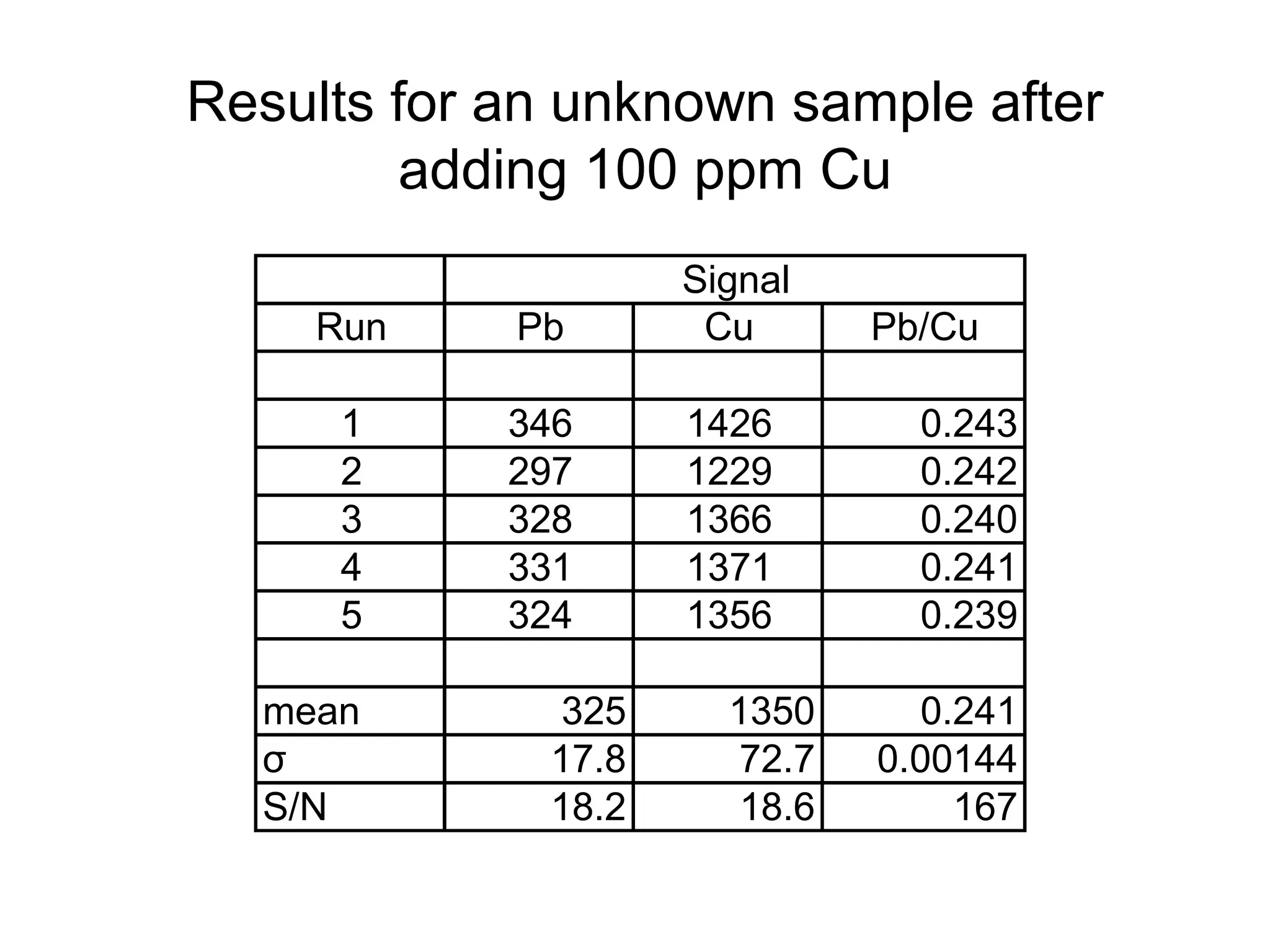
![Example: Pb by ICP Emission
Each Pb solution contains
100 ppm Cu.
Signal
[Pb]
(ppm) Pb Cu Pb/Cu
20 112 1347 0.083
40 243 1527 0.159
60 326 1383 0.236
80 355 1135 0.313
100 558 1440 0.388](https://image.slidesharecdn.com/calibration-141112131942-conversion-gate02/75/Calibration-26-2048.jpg)
![No Internal Standard Correction
600
500
400
300
200
100
0
0 20 40 60 80 100 120
[Pb] (ppm)
Pb Emission Signal](https://image.slidesharecdn.com/calibration-141112131942-conversion-gate02/75/Calibration-28-2048.jpg)
![0.450
0.400
0.350
0.300
0.250
0.200
0.150
0.100
0.050
0.000
0 20 40 60 80 100 120
[Pb] (ppm)
Pb Emission Signal
Internal Standard Correction](https://image.slidesharecdn.com/calibration-141112131942-conversion-gate02/75/Calibration-29-2048.jpg)

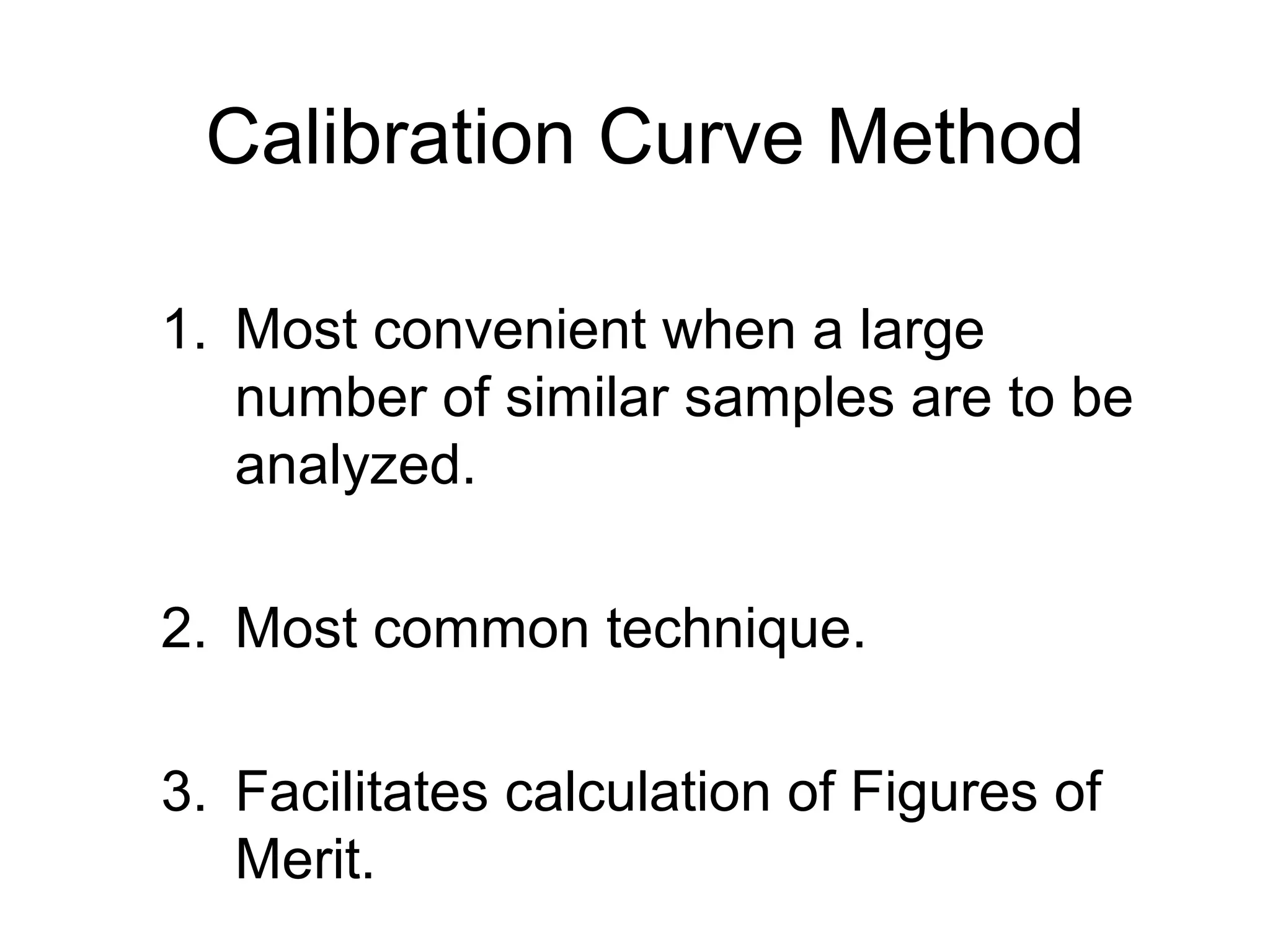
1. Three common calibration techniques are described: calibration curve method, standard additions method, and internal standard method. 2. The calibration curve method involves preparing standard solutions of a known analyte concentration and measuring the analytical signal. A calibration curve of signal vs. concentration is made to determine unknown concentrations. 3. The standard additions method is useful when sample matrix effects are present. Known amounts of standard are added to samples and the signal response is measured. The intercept of the standard additions plot indicates the original analyte concentration in the sample. 4. The internal standard method corrects for variations in sample volume, position, and matrix. A known amount of a second element is added to standards and samples. Concent


