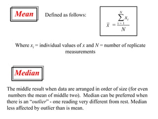
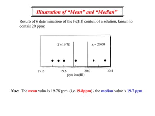
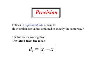
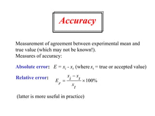
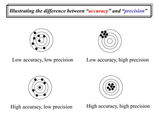
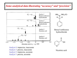
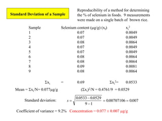
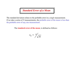
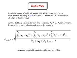
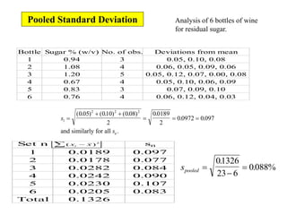
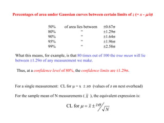
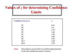
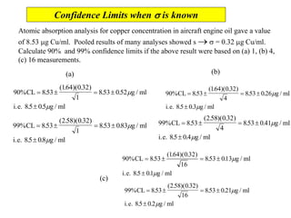
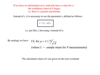
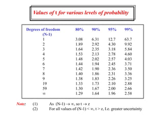
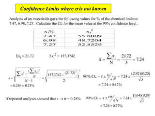
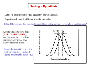
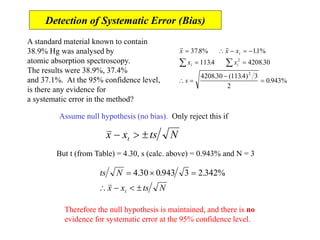
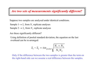
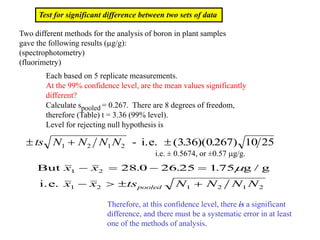
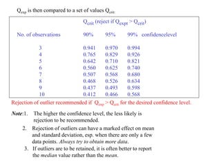
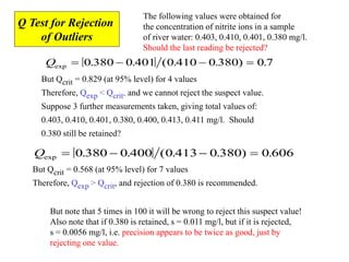
This document provides lecture notes on statistics for analytical chemistry. It begins by recommending textbooks on the subject. It then discusses various applications of analytical chemistry and outlines the general analytical problem of selecting a sample, extracting and detecting analytes, and determining the reliability of results. The notes explain the concepts of errors, precision, accuracy, and how to quantify them using statistical measures like the mean, median, and standard deviation. It provides examples of how to calculate these measures and illustrates the differences between random and systematic errors. Finally, it discusses pooling data from multiple samples to better approximate the population standard deviation.

1. Lecture Note ;
Statistics for Analytical Chemistry
(MKI 322)
Bambang Yudono
Recommended textbook:
“Statistics for Analytical Chemistry” J.C. Miller and J.N. Miller,
Second Edition, 1992, Ellis Horwood Limited
“Fundamentals of Analytical Chemistry”
Skoog, West and Holler, 7th Ed., 1996
(Saunders College Publishing)

2. Applications of Analytical Chemistry
Industrial Processes: analysis for quality control, and “reverse engineering”
(i.e. finding out what your competitors are doing).
Environmental Analysis: familiar to those who attended the second year
“Environmental Chemistry” modules. A very wide range of problems and
types of analyte
Regulatory Agencies: dealing with many problems from first two.
Academic and Industrial Synthetic Chemistry: of great interest to many of my
colleagues. I will not be dealing with this type of problem.

3. The General Analytical Problem
Select sample
Extract analyte(s) from matrix
Detect, identify and
quantify analytes
Determine reliability and
significance of results
Separate analytes

4. Errors in Chemical Analysis
Impossible to eliminate errors.
How reliable are our data?
Data of unknown quality are useless!
•Carry out replicate measurements
•Analyse accurately known standards
•Perform statistical tests on data

5. Mean Defined as follows:
x
x
N
i
N
= i = 1

Where xi = individual values of x and N = number of replicate
measurements
Median
The middle result when data are arranged in order of size (for even
numbers the mean of middle two). Median can be preferred when
there is an “outlier” - one reading very different from rest. Median
less affected by outlier than is mean.

6. Illustration of “Mean” and “Median”
Results of 6 determinations of the Fe(III) content of a solution, known to
contain 20 ppm:
Note: The mean value is 19.78 ppm (i.e. 19.8ppm) - the median value is 19.7 ppm

7. Precision
Relates to reproducibility of results..
How similar are values obtained in exactly the same way?
Useful for measuring this:
Deviation from the mean:
d x x
i i
 

8. Accuracy
Measurement of agreement between experimental mean and
true value (which may not be known!).
Measures of accuracy:
Absolute error: E = xi - xt (where xt = true or accepted value)
Relative error:
E
r
x
i
x
t
x
t


100%
(latter is more useful in practice)

9. Illustrating the difference between “accuracy” and “precision”
Low accuracy, low precision Low accuracy, high precision
High accuracy, low precision High accuracy, high precision

10. Some analytical data illustrating “accuracy” and “precision”
H
H
S
NH3+Cl-
N
H
N
OH
O
Benzyl isothiourea
hydrochloride
Nicotinic acid
Analyst 4: imprecise, inaccurate
Analyst 3: precise, inaccurate
Analyst 2: imprecise, accurate
Analyst 1: precise, accurate

11. Types of Error in Experimental
Data
Three types:
(1) Random (indeterminate) Error
Data scattered approx. symmetrically about a mean value.
Affects precision - dealt with statistically (see later).
(2) Systematic (determinate) Error
Several possible sources - later. Readings all too high
or too low. Affects accuracy.
(3) Gross Errors
Usually obvious - give “outlier” readings.
Detectable by carrying out sufficient replicate
measurements.

12. Sources of Systematic Error
1. Instrument Error
Need frequent calibration - both for apparatus such as
volumetric flasks, burettes etc., but also for electronic
devices such as spectrometers.
2. Method Error
Due to inadequacies in physical or chemical behaviour
of reagents or reactions (e.g. slow or incomplete reactions)
Example from earlier overhead - nicotinic acid does not
react completely under normal Kjeldahl conditions for
nitrogen determination.
3. Personal Error
e.g. insensitivity to colour changes; tendency to estimate
scale readings to improve precision; preconceived idea of
“true” value.

13. Systematic errors can be
constant (e.g. error in burette reading -
less important for larger values of reading) or
proportional (e.g. presence of given proportion of
interfering impurity in sample; equally significant
for all values of measurement)
Minimise instrument errors by careful recalibration and good
maintenance of equipment.
Minimise personal errors by care and self-discipline
Method errors - most difficult. “True” value may not be known.
Three approaches to minimise:
•analysis of certified standards
•use 2 or more independent methods
•analysis of blanks

14. Statistical Treatment of
Random Errors
There are always a large number of small, random errors
in making any measurement.
These can be small changes in temperature or pressure;
random responses of electronic detectors (“noise”) etc.
Suppose there are 4 small random errors possible.
Assume all are equally likely, and that each causes an error
of U in the reading.
Possible combinations of errors are shown on the next slide:

15. Combination of Random Errors
Total Error No. Relative Frequency
+U+U+U+U +4U 1 1/16 = 0.0625
-U+U+U+U +2U 4 4/16 = 0.250
+U-U+U+U
+U+U-U+U
+U+U+U-U
-U-U+U+U 0 6 6/16 = 0.375
-U+U-U+U
-U+U+U-U
+U-U-U+U
+U-U+U-U
+U+U-U-U
+U-U-U-U -2U 4 4/16 = 0.250
-U+U-U-U
-U-U+U-U
-U-U-U+U
-U-U-U-U -4U 1 1/16 = 0.01625
The next overhead shows this in graphical form

16. Frequency Distribution for
Measurements Containing Random Errors
4 random uncertainties 10 random uncertainties
A very large number of
random uncertainties
This is a
Gaussian or
normal error
curve.
Symmetrical about
the mean.

17. Replicate Data on the Calibration of a 10ml Pipette
No. Vol, ml. No. Vol, ml. No. Vol, ml
1 9.988 18 9.975 35 9.976
2 9.973 19 9.980 36 9.990
3 9.986 20 9.994 37 9.988
4 9.980 21 9.992 38 9.971
5 9.975 22 9.984 39 9.986
6 9.982 23 9.981 40 9.978
7 9.986 24 9.987 41 9.986
8 9.982 25 9.978 42 9.982
9 9.981 26 9.983 43 9.977
10 9.990 27 9.982 44 9.977
11 9.980 28 9.991 45 9.986
12 9.989 29 9.981 46 9.978
13 9.978 30 9.969 47 9.983
14 9.971 31 9.985 48 9.980
15 9.982 32 9.977 49 9.983
16 9.983 33 9.976 50 9.979
17 9.988 34 9.983
Mean volume 9.982 ml Median volume 9.982 ml
Spread 0.025 ml Standard deviation 0.0056 ml

18. Calibration data in graphical form
A = histogram of experimental results
B = Gaussian curve with the same mean value, the same precision (see later)
and the same area under the curve as for the histogram.

19. SAMPLE = finite number of observations
POPULATION = total (infinite) number of observations
Properties of Gaussian curve defined in terms of population.
Then see where modifications needed for small samples of data
Main properties of Gaussian curve:
Population mean (m) : defined as earlier (N  ). In absence of systematic error,
m is the true value (maximum on Gaussian curve).
Remember, sample mean ( x) defined for small values of N.
(Sample mean  population mean when N  20)
Population Standard Deviation (s) - defined on next overhead

20. s : measure of precision of a population of data,
given by:
s
m



( )
x
N
i
i
N
2
1
Where m = population mean; N is very large.
The equation for a Gaussian curve is defined in terms of m and s, as follows:
y
e x

 
( ) /
m s
s 
2 2
2
2

21. Two Gaussian curves with two different
standard deviations, sA and sB (=2sA)
General Gaussian curve plotted in
units of z, where
z = (x - m)/s
i.e. deviation from the mean of a
datum in units of standard
deviation. Plot can be used for
data with given value of mean,
and any standard deviation.

22. Area under a Gaussian Curve
From equation above, and illustrated by the previous curves,
68.3% of the data lie within s of the mean (m), i.e. 68.3% of
the area under the curve lies between s of m.
Similarly, 95.5% of the area lies between s, and 99.7%
between s.
There are 68.3 chances in 100 that for a single datum the
random error in the measurement will not exceed s.
The chances are 95.5 in 100 that the error will not exceed s.

23. Sample Standard Deviation, s
The equation for s must be modified for small samples of data, i.e. small N
s
x x
N
i
i
N




( )2
1
1
Two differences cf. to equation for s:
1. Use sample mean instead of population mean.
2. Use degrees of freedom, N - 1, instead of N.
Reason is that in working out the mean, the sum of the
differences from the mean must be zero. If N - 1 values are
known, the last value is defined. Thus only N - 1 degrees
of freedom. For large values of N, used in calculating
s, N and N - 1 are effectively equal.

24. Alternative Expression for s
(suitable for calculators)
s
x
x
N
N
i
i
N i
i
N







( )
( )
2
1
1
2
1
Note: NEVER round off figures before the end of the calculation

25. Reproducibility of a method for determining
the % of selenium in foods. 9 measurements
were made on a single batch of brown rice.
Sample Selenium content (mg/g) (xI) xi
2
1 0.07 0.0049
2 0.07 0.0049
3 0.08 0.0064
4 0.07 0.0049
5 0.07 0.0049
6 0.08 0.0064
7 0.08 0.0064
8 0.09 0.0081
9 0.08 0.0064
Sxi = 0.69 Sxi
2= 0.0533
Mean = Sxi/N= 0.077mg/g (Sxi)2/N = 0.4761/9 = 0.0529
Standard Deviation of a Sample
s 


 
00533 00529
9 1
0 00707106 0007
. .
. .
Coefficient of variance = 9.2% Concentration = 0.077 ± 0.007 mg/g
Standard deviation:

26. Standard Error of a Mean
The standard deviation relates to the probable error in a single measurement.
If we take a series of N measurements, the probable error of the mean is less than
the probable error of any one measurement.
The standard error of the mean, is defined as follows:
s s
N
m 

27. Pooled Data
To achieve a value of s which is a good approximation to s, i.e. N  20,
it is sometimes necessary to pool data from a number of sets of measurements
(all taken in the same way).
Suppose that there are t small sets of data, comprising N1, N2,….Nt measurements.
The equation for the resultant sample standard deviation is:
s
x x x x x x
N N N t
pooled
i i i
i
N
i
N
i
N

     
   





( ) ( ) ( ) ....
......
1
2
2
2
3
2
1
1
1
1 2 3
3
2
1
(Note: one degree of freedom is lost for each set of data)

28. Analysis of 6 bottles of wine
for residual sugar.
Bottle Sugar % (w/v) No. of obs. Deviations from mean
1 0.94 3 0.05, 0.10, 0.08
2 1.08 4 0.06, 0.05, 0.09, 0.06
3 1.20 5 0.05, 0.12, 0.07, 0.00, 0.08
4 0.67 4 0.05, 0.10, 0.06, 0.09
5 0.83 3 0.07, 0.09, 0.10
6 0.76 4 0.06, 0.12, 0.04, 0.03
s
sn
1
2 2 2
0 05 010 0 08
2
0 0189
2
0 0972 0 097

 
  
( . ) ( . ) ( . ) .
. .
and similarly for all .
Set n sn
1 0.0189 0.097
2 0.0178 0.077
3 0.0282 0.084
4 0.0242 0.090
5 0.0230 0.107
6 0.0205 0.083
Total 0.1326
( )
x x
i
  2
spooled 


01326
23 6
0088%
.
.
Pooled Standard Deviation

29. Two alternative methods for measuring the precision of a set of results:
VARIANCE: This is the square of the standard deviation:
s
x x
N
i
i
N
2
2 2
1
1




( )
COEFFICIENT OF VARIANCE (CV)
(or RELATIVE STANDARD DEVIATION):
Divide the standard deviation by the mean value and express as a percentage:
CV
s
x
 
( ) 100%

30. Use of Statistics in Data
Evaluation

31. How can we relate the observed mean value ( x ) to the true mean (m)?
The latter can never be known exactly.
The range of uncertainty depends how closely s corresponds to s.
We can calculate the limits (above and below) around x that m must lie,
with a given degree of probability.

32. Define some terms:
CONFIDENCE LIMITS
interval around the mean that probably contains m.
CONFIDENCE INTERVAL
the magnitude of the confidence limits
CONFIDENCE LEVEL
fixes the level of probability that the mean is within the confidence limits
Examples later. First assume that the known s is a good
approximation to s.

33. Percentages of area under Gaussian curves between certain limits of z (= x - m/s)
50% of area lies between 0.67s
80% “ 1.29s
90% “ 1.64s
95% “ 1.96s
99% “ 2.58s
What this means, for example, is that 80 times out of 100 the true mean will lie
between 1.29s of any measurement we make.
Thus, at a confidence level of 80%, the confidence limits are 1.29s.
For a single measurement: CL for m = x  zs (values of z on next overhead)
For the sample mean of N measurements ( x ), the equivalent expression is:
CL for m s
 
x z
N

34. Values of z for determining Confidence
Limits
Confidence level, % z
50 0.67
68 1.0
80 1.29
90 1.64
95 1.96
96 2.00
99 2.58
99.7 3.00
99.9 3.29
Note: these figures assume that an excellent approximation
to the real standard deviation is known.

35. Atomic absorption analysis for copper concentration in aircraft engine oil gave a value
of 8.53 mg Cu/ml. Pooled results of many analyses showed s  s = 0.32 mg Cu/ml.
Calculate 90% and 99% confidence limits if the above result were based on (a) 1, (b) 4,
(c) 16 measurements.
90% 853
164 032
1
853 052
85 05
CL g / ml
i.e. g / ml
   

.
( . )( . )
. .
. .
m
m
(a)
99% 853
258 032
1
853 083
85 08
CL g / ml
i.e. g / ml
   

.
( . )( . )
. .
. .
m
m
(b)
90% 853
164 032
4
853 026
85 03
CL g / ml
i.e. g / ml
   

.
( . )( . )
. .
. .
m
m
99% 853
258 032
4
853 041
85 04
CL g / ml
i.e. g / ml
   

.
( . )( . )
. .
. .
m
m
(c)
90% 853
164 0 32
16
853 013
85 01
CL g / ml
i.e. g / ml
   

.
( . )( . )
. .
. .
m
m
99% 853
258 032
16
853 021
85 02
CL g / ml
i.e. g / ml
   

.
( . )( . )
. .
. .
m
m
Confidence Limits when s is known

36. If we have no information on s, and only have a value for s -
the confidence interval is larger,
i.e. there is a greater uncertainty.
Instead of z, it is necessary to use the parameter t, defined as follows:
t = (x - m)/s
i.e. just like z, but using s instead of s.
By analogy we have: CL for
(where = sample mean for measurements)
m  
x ts
N
x N
The calculated values of t are given on the next overhead

37. Values of t for various levels of probability
Degrees of freedom 80% 90% 95% 99%
(N-1)
1 3.08 6.31 12.7 63.7
2 1.89 2.92 4.30 9.92
3 1.64 2.35 3.18 5.84
4 1.53 2.13 2.78 4.60
5 1.48 2.02 2.57 4.03
6 1.44 1.94 2.45 3.71
7 1.42 1.90 2.36 3.50
8 1.40 1.86 2.31 3.36
9 1.38 1.83 2.26 3.25
19 1.33 1.73 2.10 2.88
59 1.30 1.67 2.00 2.66
 1.29 1.64 1.96 2.58
Note: (1) As (N-1)  , so t  z
(2) For all values of (N-1) < , t > z, I.e. greater uncertainty

38. Analysis of an insecticide gave the following values for % of the chemical lindane:
7.47, 6.98, 7.27. Calculate the CL for the mean value at the 90% confidence level.
xi% xi
2
7.47 55.8009
6.98 48.7204
7.27 52.8529
Sxi = 21.72 Sxi
2 = 157.3742
x
x
N
i
  
 2172
3
7 24
.
.
s
x
x
N
N
i
i





 

 2
2
2
1
157 3742
2172
3
2
0 246 0 25%
( )
.
( . )
. .
90% CL    
 
x ts
N
7 24
2 92 0 25
3
7 24 0 42%
.
( . )( . )
. .
If repeated analyses showed that s s = 0.28%: 90% CL    
 
x z
N
s 7 24
164 0 28
3
7 24 0 27%
.
( . )( . )
. .
Confidence Limits where s is not known

39. Testing a Hypothesis
Carry out measurements on an accurately known standard.
Experimental value is different from the true value.
Is the difference due to a systematic error (bias) in the method - or simply to random error?
Assume that there is no bias
(NULL HYPOTHESIS),
and calculate the probability
that the experimental error
is due to random errors.
Figure shows (A) the curve for
the true value (mA = mt) and
(B) the experimental curve (mB)

40. Bias = mB- mA = mB - xt.
Test for bias by comparing with the
difference caused by random error
x xt

Remember confidence limit for m (assumed to be xt, i.e. assume no bias)
is given by:
CL for
at desired confidence level, random
errors can lead to:
if , then at the desired
confidence level bias (systematic error)
is likely (and vice versa).
m  

  
  
x
ts
N
x x
ts
N
x x
ts
N
t
t

41. A standard material known to contain
38.9% Hg was analysed by
atomic absorption spectroscopy.
The results were 38.9%, 37.4%
and 37.1%. At the 95% confidence level,
is there any evidence for
a systematic error in the method?
x x x
x x
s
t
i i
    
 
 


 
37 8% 11%
1134 4208 30
4208 30 1134 3
2
0 943%
2
2
. .
. .
. ( . )
.
Assume null hypothesis (no bias). Only reject this if
x x ts N
t
  
But t (from Table) = 4.30, s (calc. above) = 0.943% and N = 3
ts N
x x ts N
t
  
   
4 30 0 943 3 2 342%
. . .
Therefore the null hypothesis is maintained, and there is no
evidence for systematic error at the 95% confidence level.
Detection of Systematic Error (Bias)

42. Are two sets of measurements significantly different?
Suppose two samples are analysed under identical conditions.
Sample 1 from replicate analyses
Sample 2 from replicate analyses


x N
x N
1 1
2 2
Are these significantly different?
Using definition of pooled standard deviation, the equation on the last
overhead can be re-arranged:
x x ts
N N
N N
pooled
1 2
1 2
1 2
  

Only if the difference between the two samples is greater than the term on
the right-hand side can we assume a real difference between the samples.

43. Test for significant difference between two sets of data
Two different methods for the analysis of boron in plant samples
gave the following results (mg/g):
(spectrophotometry)
(fluorimetry)
Each based on 5 replicate measurements.
At the 99% confidence level, are the mean values significantly
different?
Calculate spooled = 0.267. There are 8 degrees of freedom,
therefore (Table) t = 3.36 (99% level).
Level for rejecting null hypothesis is
  
ts N N N N
1 2 1 2 336 0 267 10 25
- i.e. ( . )( . )
i.e. ± 0.5674, or ±0.57 mg/g.
But g / g
x x
1 2 28 0 26 25 1 75
   
. . . m
i.e. x x ts N N N N
pooled
1 2 1 2 1 2
   
Therefore, at this confidence level, there is a significant
difference, and there must be a systematic error in at least
one of the methods of analysis.

44. A set of results may contain an outlying result
- out of line with the others.
Should it be retained or rejected?
There is no universal criterion for deciding this.
One rule that can give guidance is the Q test.

Qexp  xq  xn /w
where xq = questionable result
xn = nearest neighbour
w = spread of entire set
Consider a set of results
The parameter Qexp is defined as follows:
Detection of Gross Errors

45. Qexp is then compared to a set of values Qcrit:
Rejection of outlier recommended if Qexp > Qcrit for the desired confidence level.
Note:1. The higher the confidence level, the less likely is
rejection to be recommended.
2. Rejection of outliers can have a marked effect on mean
and standard deviation, esp. when there are only a few
data points. Always try to obtain more data.
3. If outliers are to be retained, it is often better to report
the median value rather than the mean.
Qcrit (reject if Qexpt > Qcrit)
No. of observations 90% 95% 99% confidencelevel
3 0.941 0.970 0.994
4 0.765 0.829 0.926
5 0.642 0.710 0.821
6 0.560 0.625 0.740
7 0.507 0.568 0.680
8 0.468 0.526 0.634
9 0.437 0.493 0.598
10 0.412 0.466 0.568

46. The following values were obtained for
the concentration of nitrite ions in a sample
of river water: 0.403, 0.410, 0.401, 0.380 mg/l.
Should the last reading be rejected?
Qexp . . ( . . ) .
   
0 380 0 401 0 410 0 380 0 7
But Qcrit = 0.829 (at 95% level) for 4 values
Therefore, Qexp < Qcrit, and we cannot reject the suspect value.
Suppose 3 further measurements taken, giving total values of:
0.403, 0.410, 0.401, 0.380, 0.400, 0.413, 0.411 mg/l. Should
0.380 still be retained?
Qexp . . ( . . ) .
   
0 380 0 400 0 413 0 380 0 606
But Qcrit = 0.568 (at 95% level) for 7 values
Therefore, Qexp > Qcrit, and rejection of 0.380 is recommended.
But note that 5 times in 100 it will be wrong to reject this suspect value!
Also note that if 0.380 is retained, s = 0.011 mg/l, but if it is rejected,
s = 0.0056 mg/l, i.e. precision appears to be twice as good, just by
rejecting one value.
Q Test for Rejection
of Outliers

47. Obtaining a representative sample
Homogeneous gaseous or liquid sample
No problem – any sample representative.
Solid sample - no gross heterogeneity
Take a number of small samples at random from throughout the bulk - this will
give a suitable representative sample.
Solid sample - obvious heterogeneity
Take small samples from each homogeneous region and
mix these in the same proportions as between each
region and the whole.
If it is suspected, but not certain, that a bulk material is heterogeneous, then
it is necessary to grind the sample to a fine powder, and mix this very
thoroughly before taking random samples from the bulk.
For a very large sample - a train-load of metal ore, or soil in a field - it is always
necessary to take a large number of random samples from throughout the whole.

48. Sample Preparation
and Extraction
May be many analytes present - separation - see later.
May be small amounts of analyte(s) in bulk material.
Need to concentrate these before analysis.e.g. heavy metals in
animal tissue, additives in polymers, herbicide residues in flour etc. etc.
May be helpful to concentrate complex mixtures selectively.
Most general type of pre-treatment: EXTRACTION.

49. Classical extraction method is: SOXHLET EXTRACTION
(named after developer).
Apparatus
Sample in porous
thimble.
Exhaustive reflux for
up to 1 - 2 days.
Solution of analyte(s)
in volatile solvent
(e.g. CH2Cl2, CHCl3 etc.)
Evaporate to dryness or
suitable concentration,
for separation/analysis.