Downloaded 158 times
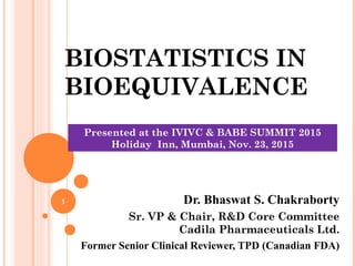
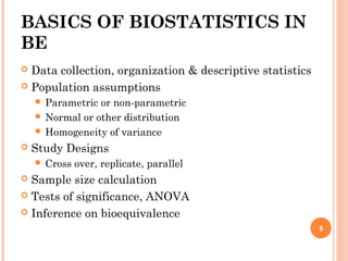
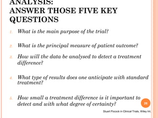
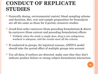
![FROM THE PREVIOUS
GRAPH, WE HAVE
0+Z1-α/2σ√(2/N) = δ–Z1-βσ√(2/N)
Upon simplification,
N =
2 σ2
[Z1-α/2 + Z1-β/2]2
δ 2
25](https://image.slidesharecdn.com/biostatisticsinbe23nov2015final-151207075706-lva1-app6891/85/Biostatistics-in-Bioequivalence-25-320.jpg)
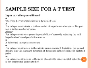
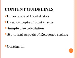
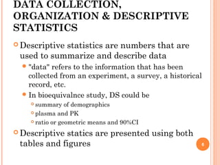
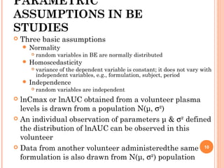
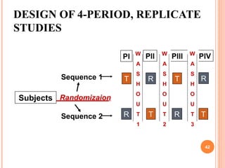
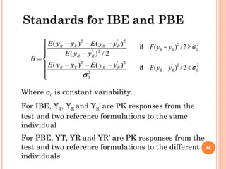
![31
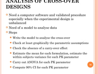
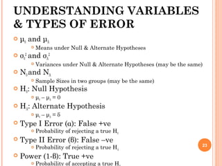
• The hypotheses to be tested:
• The equivalence interval : [0.8, 1.25]
• The experimental design : crossover (2×2) with the same
number of subjects per sequence N
• The consumer risk (α = 5%)
• The producer/trialist risk (β = 20%)
• A log transformation is required
• An estimate of intra-subject variation from
log-transformed data)
• An estimate of µT/µR
DETERMINING BE SAMPLE
SIZE
25.18.0 ≤≤
R
T
µ
µ multiplicative](https://image.slidesharecdn.com/biostatisticsinbe23nov2015final-151207075706-lva1-app6891/85/Biostatistics-in-Bioequivalence-31-320.jpg)

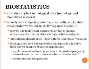
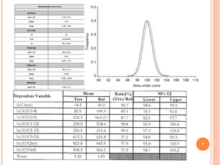
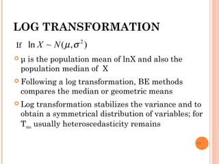
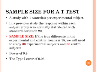
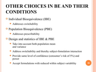
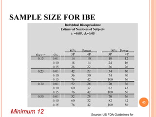
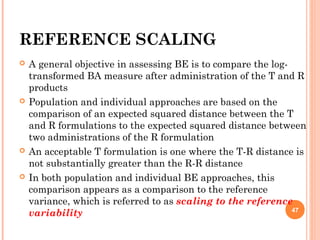
![33
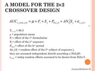
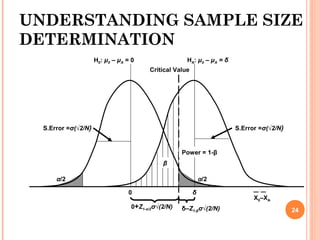
SAMPLE SIZE BE
µT/µR
CV % 0.85 0.90 0.95 1.00 1.05 1.10 1.15 1.20
5.0% 12 6 4 4 4 6 8 22
7.5% 22 8 6 6 6 8 12 44
10.0% 36 12 8 6 8 10 20 76
12.5% 54 16 10 8 10 14 30 118
15.0% 78 22 12 10 12 20 42 168
Number of subjects per sequence for a 2×2 crossover,
log transformation, equivalence interval : [0.8, 1.25],
α=5%, β = 20%](https://image.slidesharecdn.com/biostatisticsinbe23nov2015final-151207075706-lva1-app6891/85/Biostatistics-in-Bioequivalence-33-320.jpg)


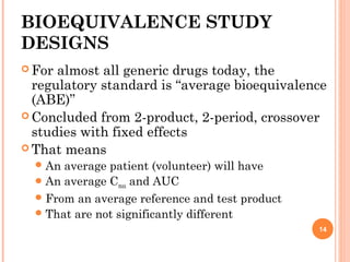
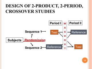
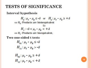
This document discusses biostatistics in bioequivalence studies. It covers: 1) The importance of biostatistics in designing and analyzing bioequivalence trials, as well as distinguishing between correlation and causation. 2) Key biostatistical concepts for bioequivalence studies including descriptive statistics, parametric assumptions of normality and homoscedasticity, study designs, and tests of significance. 3) Details on sample size calculation and determining the number of subjects needed in a bioequivalence study based on factors like variability, equivalence bounds, type I and II error rates.


![How Big Brands are Taking Your Traffic in Alberta [Data Inside].pptx](https://cdn.slidesharecdn.com/ss_thumbnails/howbigbrandsaretakingyourtrafficinalbertadatainside-260123180142-42d276f3-thumbnail.jpg?width=640&height=640&fit=bounds)


