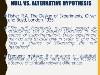
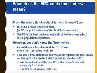
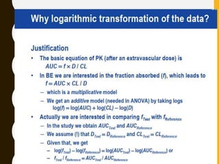
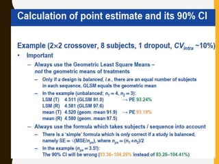
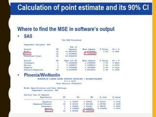
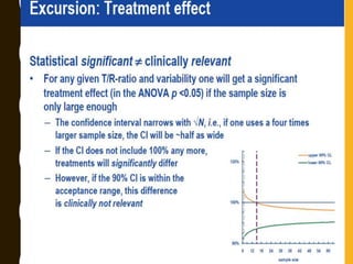
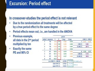
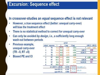
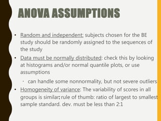
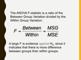
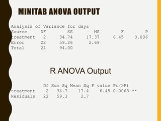
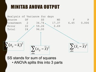
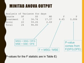
The document discusses statistical methods for determining sample sizes and analyzing pharmacokinetic (PK) measures to assess bioequivalence between test and reference formulations. It emphasizes the importance of hypothesis testing, outlining conventional methods and the inadequacies associated with them, particularly regarding conclusions on equality. Additionally, it details procedures for analyzing data using ANOVA and the factors influencing sample size calculations in bioequivalence studies.

1. STATISTICAL METHODS
AND DETERMINATION OF
SAMPLE SIZE
PRESENTED B Y
SALUM MKATA
R.PHARM.

3. • Statistical analyses of PK measures (e.g.,
AUC ad Cmax) based on two one-sided
tests procedure to determine whether the
mean PK values for T & R are comparable
• BE concluded if the 90% CI for the ratio of
geometric means for T & R is within limits
of 80 – 125% (exceptions)
STATISTICAL ANALYSIS

4. TO SOLVE THIS NIGHTMARE
LET STARTS WITH THIS………
HYPOTHESIS TESTING AND CONFIDENCE INTERVAL

5. HYPOTHESIS TEST
 Convectional hypothesis test (frequentist statistics)
- Ho: θ= θ1 H1: θ≠ θ1 (in this case it is two-sided)
 Usually expressed as a difference: Ho: d= 0, H1: d≠ 0
-If P<0.05 we can conclude that statistical significant difference exists
-If P>0.05 we cannot conclude
• With the available potency we cannot detect a difference
• But it does not mean that the difference does not exist
• And it does not mean that they are equivalent or equal
 We only have certainty when we reject the null hypothesis
-In superiority trials: H1 is for existence of differences
 This conventional test is inadequate to conclude about “equalities”
-In fact, it is impossible to conclude “equality”

6. NULL VS. ALTERNATIVE HYPOTHESIS
 Fisher, R.A. The Design of Experiments, Oliver
and Boyd, London, 1935
 “The null hypothesis is never proved or
established, but is possibly disproved in the
course of experimentation. Every experiment
may be said to exist only in order to give the
facts a chance of disproving the null
hypothesis”
 Frequent mistake: the absence of statistical
significance has been interpreted incorrectly as
absence of clinically relevant differences

7. (BIO) EQUIVALENCE
 We are interested in verifying (instead of rejecting)
the null hypothesis of a conventional hypothesis
test
 We have to redefine the alternative hypothesis as a
range of values with an equivalent effect
 The differences within this range are considered clinically irrelevant
 Problem: It's very difficult to define the maximum
difference without clinical relevance for the Cmax
and AUC of each drug
 Solution: 20% difference considered clinically
irrelevant based on a survey among physicians in
1970s.

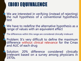
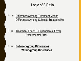
8. INTERVAL HYPOTHESIS OR TWO ONE-
SIDED TESTS
 Redefine the null hypothesis: How?
 Solution: It is like changing the null to the alternative
hypothesis and vice versa.
 Alternative hypothesis test: Schuirmann, 1981
 This is equivalent to:
H 0 : T - R < D1 or T - R > D2
H A : D1  T - R  D2
 It is called as an interval hypothesis because the equivalence hypothesis is in
the alternative hypothesis and it is expressed as an interval
bioequivalence
bioinequivalence
T and R population mean for test and reference
formulation respectively
[D1 ; D2] Absolute equivalence
interval
H 0 : T - R < D1
H 0 : T - R > D2
H A : D1  T - R
H A : T - R  D2

9. INTERVAL HYPOTHESIS OR TWO ONE-
SIDED TESTS
 The new alternative hypothesis is decided with a
statistic that follows a distribution that can be
approximated to a t-distribution
 To conclude bioequivalence a P value <0.05 has
to be obtained in both one-sided tests
 The hypothesis tests do not give an idea of
magnitude of equivalence (P<0.001 vs. 90% CI:
0.95 – 1.05).
 That is why confidence intervals are preferred
Source: Slides from Dr. Alfredo Garcia – Addis Ababa, Ethiopia 2010

10. THE TWO ONE-SIDED TESTS
(SCHUIRMAN)
10
bioequivalence
H 0 : T - R < D1 or T - R > D2
H A : D1  T - R  D2
H 0 : T - R < D1
H A : D1  T - R
H 0 : T - R > D2
H A : T - R  D2
First one-sided test second one-sided test
Bioequivalence when the 2 tests reject H0

11. EQUIVALENCE STUDY
d < 0
Negative effect
d = 0
No difference
d > 0
Positive effect
-d +d
Region of
clinical
equivalence
Slides from Dr. Alfredo Garcia – Addis Ababa, Ethiopia 2010

26. ANOVA MODEL
•Non replicate designs
–General linear model procedure (PROC GLM)
–Linear mixed effects model procedure (PROC
MIXED)
•Replicate crossover designs
–Linear mixed effects procedure (PROC MIXED)
NB: For parallel and replicate designs – do not
assume equal variances.

27. ANOVA MODEL – MULTIPLE GROUPS
• Multiple groups
– Model should be modified to reflect the group nature
– e.g. reflect that the periods of 1st group are different
from those of the second group.
– 2 groups from different sites or same site but separated
by longer period e.g. months: results may not be
combined in single analysis
• Sequential design: where decision for 2nd group is based on
results of the 1st group- different statistical methods are
required

28. WHAT DOES ANOVA DO?
At its simplest (there are extensions)
ANOVA tests the following hypotheses:
H0: The means of all the groups are equal.
Ha: Not all the means are equal
• doesn’t say how or which ones differ.
• Can follow up with “multiple
comparisons”
Note: we usually refer to the sub-populations
as “groups” when doing ANOVA.

29. ANOVA ASSUMPTIONS
• Random and independent: subjects chosen for the BE
study should be randomly assigned to the sequences of
the study
• Data must be normally distributed: check this by looking
at histograms and/or normal quantile plots, or use
assumptions
· can handle some nonnormality, but not severe outliers
• Homogeneity of variance: The variability of scores in all
groups is similar; rule of thumb: ratio of largest to smallest
sample standard. dev. must be less than 2:1

30. NOTATION FOR ANOVA
• n = number of individuals all together
• I = number of groups
• = mean for entire data set is
Group i has
• ni = # of individuals in group i
• xij = value for individual j in group i
• = mean for group i
• si = standard deviation for group i

31. HOW ANOVA WORKS (OUTLINE)
ANOVA measures two sources of variation in the data and
compares their relative sizes
• variation BETWEEN groups
• for each data value look at the difference between
its group mean and the overall mean
• variation WITHIN groups
• for each data value we look at the difference
between that value and the mean of its group

32. Sum of Squared Deviations
Total Sum of Squares = Sum of Squared between-group
deviations + Sum of Squared within-group deviations
SSTotal = SSBetween + SSWithinb

33. The ANOVA F-statistic is a ratio of the
Between Group Variation divided by the
Within Group Variation:
A large F is evidence against H0, since it
indicates that there is more difference
between groups than within groups.

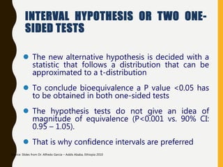
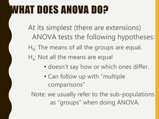
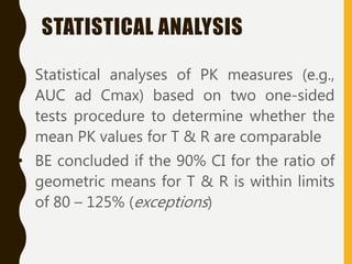
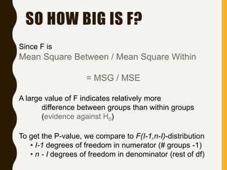
34. AN EXAMPLE ANOVA
SITUATION
Subjects: 25 patients with blisters
Treatments: Treatment A, Treatment B, Placebo
Measurement: # of days until blisters heal
Data [and means]:
• A: 5,6,6,7,7,8,9,10 [7.25]
• B: 7,7,8,9,9,10,10,11 [8.875]
• P: 7,9,9,10,10,10,11,12,13 [10.11]
Are these differences significant?

35. MINITAB ANOVA OUTPUT
Analysis of Variance for days
Source DF SS MS F P
treatment 2 34.74 17.37 6.45 0.006
Error 22 59.26 2.69
Total 24 94.00
Df Sum Sq Mean Sq F value Pr(>F)
treatment 2 34.7 17.4 6.45 0.0063 **
Residuals 22 59.3 2.7
R ANOVA Output

36. MINITAB ANOVA OUTPUT
Analysis of Variance for days
Source DF SS MS F P
treatment 2 34.74 17.37 6.45 0.006
Error 22 59.26 2.69
Total 24 94.00
SS stands for sum of squares
• ANOVA splits this into 3 parts

37. MINITAB ANOVA OUTPUT
MSG = SSG / DFG
MSE = SSE / DFE
Analysis of Variance for days
Source DF SS MS F P
treatment 2 34.74 17.37 6.45 0.006
Error 22 59.26 2.69
Total 24 94.00
F = MSG / MSE
P-value
comes from
F(DFG,DFE)
(P-values for the F statistic are in Table E)

38. F = Differences Among Treatment Means
Differences Among Subjects Treated Alike
F = Treatment Effect + (Experimental Error)
Experimental Error
F = Between-group Differences
Within-group Differences
Logic of F Ratio

39. SO HOW BIG IS F?
Since F is
Mean Square Between / Mean Square Within
= MSG / MSE
A large value of F indicates relatively more
difference between groups than within groups
(evidence against H0)
To get the P-value, we compare to F(I-1,n-I)-distribution
• I-1 degrees of freedom in numerator (# groups -1)
• n - I degrees of freedom in denominator (rest of df)

40. WHERE’S THE DIFFERENCE?
Analysis of Variance for days
Source DF SS MS F P
treatment 2 34.74 17.37 6.45 0.006
Error 22 59.26 2.69
Total 24 94.00
Individual 95% CIs For Mean
Based on Pooled StDev
Level N Mean StDev ----------+---------+---------+------
A 8 7.250 1.669 (-------*-------)
B 8 8.875 1.458 (-------*-------)
P 9 10.111 1.764 (------*-------)
----------+---------+---------+------
Pooled StDev = 1.641 7.5 9.0 10.5
Once ANOVA indicates that the groups do not all
appear to have the same means, what do we do?
Clearest difference: P is worse than A (CI’s don’t overlap)

41. Logic of F Test and Hypothesis Testing
Form of F Test: Between Group Differences
Within Group Differences
Purpose: Test null hypothesis: Between Group = Within Group =
Random Error
Interpretation: If null hypothesis is not supported (F > 1) then
Between Group diffs are not simply random error, but
instead reflect effect of the independent variable.
Result: Null hypothesis is rejected, alt. hypothesis is
supported
(BUT NOT PROVED!)

42. REMEMBER THIS

43. Sample size in BE Studies

44. AT THE END OF THE
SESSION…
You should be able to:
• Recognise the key factors in
calculation of sample size for BE
studies;
• Integrate the concepts for sample size
determination in the overall design of
the study.

45. ACKNOWLEDGEMENTS
• Slides adopted from Dr Alfredo Garcia
Presentations
10/10/2021 45

46. HOW TO CALCULATE THE SAMPLE
SIZE OF A 2X2 CROSS-OVER
BIOEQUIVALENCE STUDY

47. FACTORS AFFECTING THE SAMPLE SIZE
• The error variance (CV%) of the primary PK
parameters
– Published data
– Pilot study
• The significance level desired (5%): consumer’s risk
• The statistical power desired (>80%): producer’s risk
• The expected mean deviation from comparator
• The acceptance criteria: (usually 80-125% or ±20%)

48. REASONS FOR A CORRECT CALCULATION OF
THE SAMPLE SIZE
• Too many subjects
– It is unethical to expose more subjects than necessary
– Unnecessary risk for some subjects
– It is an unnecessary waste of some resources ($)
• Too few subjects
– A study unable to reach its objective is unethical
– All subjects at risk for nothing
– All resources ($) is wasted when the study is
inconclusive
• Minimum number of subjects: 12

49. FREQUENT MISTAKES
• To calculate the sample size required to detect a 20%
difference assuming that treatments are e.g. equal
– Pocock, Clinical Trials, 1983
• To use calculation based on data without log-
transformation
– Design and Analysis of Bioavailability and Bioequivalence
Studies, Chow & Liu, 1992 (1st edition) and 2000 (2nd edition)
• Too many extra subjects. Usually no need of more than
10%. Depends on tolerability
– 10% proposed by Patterson et al, Eur J Clin Pharmacol 57: 663-
670 (2001)

50. • Exact value has to be obtained with power curves
• Approximate values are obtained based on
formulae
–Best approximation: iterative process (t-test)
–Acceptable approximation: based on Normal
distribution
• Calculations are different when we assume
products are really equal and when we assume
products are slightly different
• Any minor deviation is masked by extra subjects to
be included to compensate drop-outs and
withdrawals (10%)
METHODS TO CALCULATE THE
SAMPLE SIZE

51. 51
• Both treatments are equal
SAMPLE SIZE CALCULATION
 
 
 2
2
1
2
1
2
25
.
1
2
Ln
Z
Z
s
N
w 
 
 



 
   
 2
2
1
1
2
25
.
1
2
Ln
Ln
Z
Z
s
N
R
T
w




 





• Assumptions on difference between treatments
• Treatments are different
1

R
T 
 1

R
T 

 
2
2
1 CV
Ln
sw 

CV expressed as 0.3 for 30%

52. • Calculation assuming that
treatments are equal
ASSUMPTIONS ON DIFFERENCE BETWEEN
TREATMENTS
 
 
 2
2
1
2
1
2
25
.
1
2
Ln
Z
Z
s
N
w 
 
 



 
   
 2
2
1
1
2
25
.
1
2
Ln
Ln
Z
Z
s
N
R
T
w




 





• Z(1-(/2)) = DISTR.NORM.ESTAND.INV(0.05) for
90% 1-
• Z(1-(/2)) = DISTR.NORM.ESTAND.INV(0.1) for 80%
1-
• Z(1- ) = DISTR.NORM.ESTAND.INV(0.05) for 5% 
• Calculation assuming that
treatments are not equal
Z(1-) = DISTR.NORM.ESTAND.INV(0.1) for 90% 1-
Z(1-) = DISTR.NORM.ESTAND.INV(0.2) for 80% 1-
Z(1-) = DISTR.NORM.ESTAND.INV(0.05) for 5% 

53. QUESTIONS
?