Download as PDF, PPTX
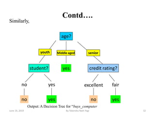
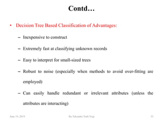
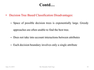
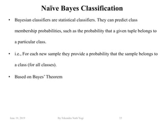
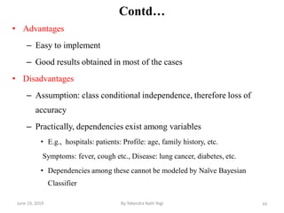
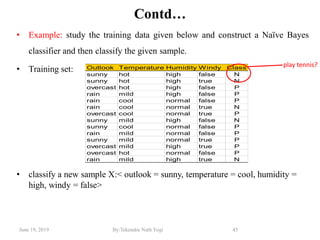
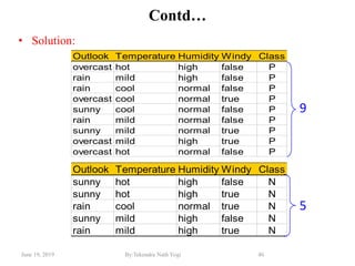
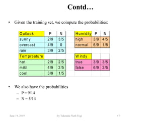
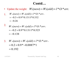
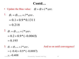


The document discusses various classification techniques used in data analysis, including decision tree classifiers, rule-based classifiers, and Bayesian classifiers. It covers when to use classification versus prediction, the process of building classifiers, and the importance of testing model accuracy to avoid overfitting. The document also highlights the advantages and disadvantages of decision tree methods and introduces basic concepts of naive Bayes classification.


![Getting Started with Apache Spark: Big Data Made Simple [Free Meetup]](https://cdn.slidesharecdn.com/ss_thumbnails/apachesparkgettingstarted-260203175547-8361bcc3-thumbnail.jpg?width=640&height=640&fit=bounds)

