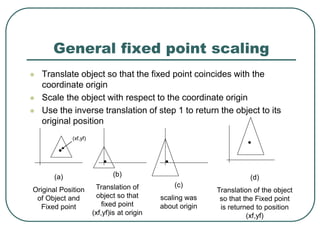
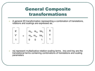
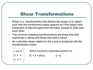
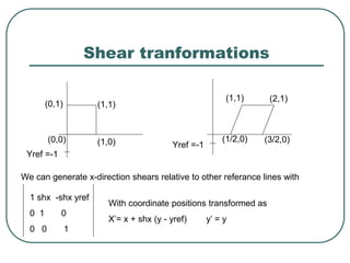
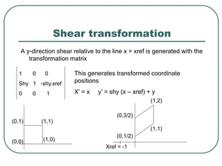
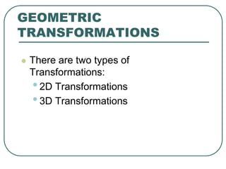
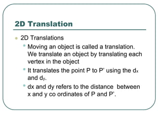
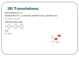
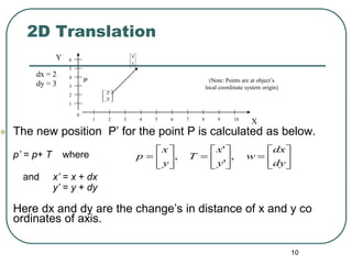
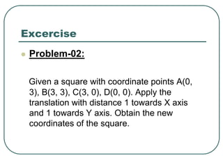
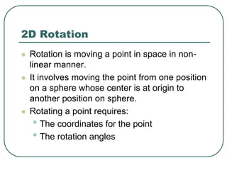
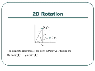
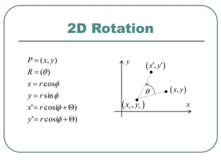
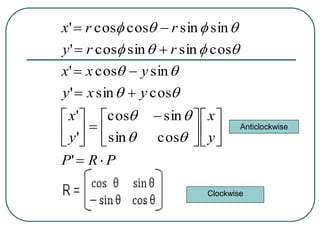
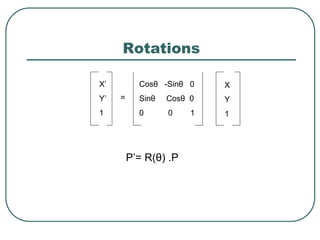
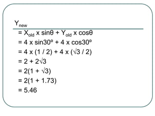
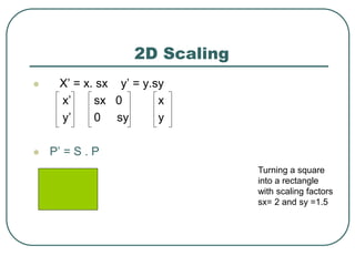
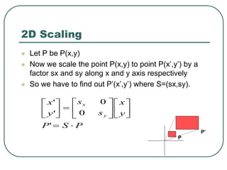
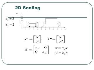
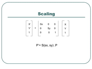
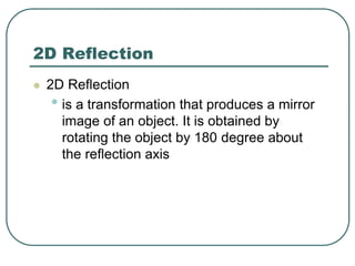
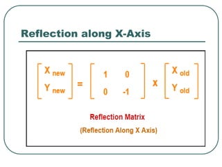
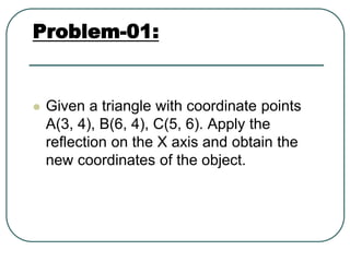
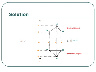
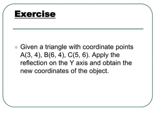
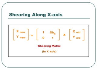
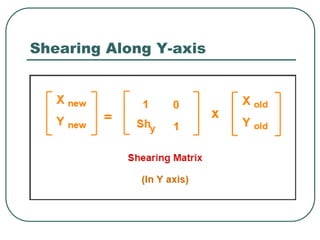
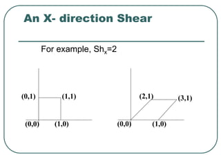
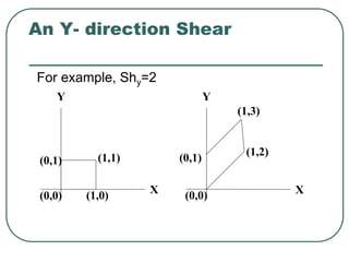
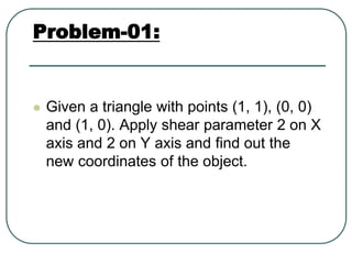
Geometric transformations play an important role in computer graphics by allowing graphics to be repositioned on the screen or changed in size and orientation. There are several types of 2D transformations including translation, rotation, scaling, reflection, and shearing. Translation moves an object by translating each vertex by a certain distance. Rotation moves a point around a center point by a certain angle. Scaling enlarges or shrinks an object by a scaling factor. Reflection produces a mirror image of an object across an axis. Shearing distorts an object by shifting coordinate values.

1. TRANSFORMATIONS
Dr Bharti Sharma

2. Transformation
In Computer graphics, Transformation is a
process of modifying and re-positioning
the existing graphics.

3. Transformation
 Transformation means changing some graphics into
something else by applying rules. We can have
various types of transformations such as translation,
scaling up or down, rotation, shearing, etc. When a
transformation takes place on a 2D plane, it is called
2D transformation.
 Transformations play an important role in computer
graphics to reposition the graphics on the screen
and change their size or orientation.

4. GEOMETRIC
TRANSFORMATIONS
Geometric Transformation
 The object itself is moved relative to a stationary
coordinate system or background.
 With respect to some 2-D coordinate system, an
object O is considered as a set of points.
O = { P(x,y)}
 If the Object O moves to a new position, the new
object O’ is considered:
O’ = { P’(x’,y’)}

5. GEOMETRIC
TRANSFORMATIONS
 There are two types of
Transformations:
•2D Transformations
•3D Transformations

7. 2D Translation
 2D Translations
• Moving an object is called a translation.
We translate an object by translating each
vertex in the object
• It translates the point P to P’ using the dx
and dy.
• dx and dy refers to the distance between
x and y co ordinates of P and P’.

8. 2D Translation
x’= x + tx
y’= y + ty
The translation distance pair (tx,ty) is called a
translation vector or shift vector
P = x1 P’= x1’ T = tx
x2 x2’ ty
This allows us to write the two dimensional translation
equations in the matrix form
P’ = P + T

9. 2D Translations

10. 10
•
P
 The new position P’ for the point P is calculated as below.
p’ = p+ T where
and x’ = x + dx
y’ = y + dy
Here dx and dy are the change’s in distance of x and y co
ordinates of axis.
2D Translation
dx = 2
dy = 3
Y
X
0
1
1
2
2
3 4 5 6 7 8 9 10
3
4
5
6





















dy
dx
w
y
x
T
y
x
p ,
'
'
,






2
2






5
4
(Note: Points are at object’s
local coordinate system origin)

12. Translation
 Problem-01:
Given a circle C with radius 10 and center
coordinates (1, 4). Apply the translation with distance
5 towards X axis and 1 towards Y axis. Obtain the
new coordinates of C without changing its radius.

13. Solution

14. Excercise
 Problem-02:
Given a square with coordinate points A(0,
3), B(3, 3), C(3, 0), D(0, 0). Apply the
translation with distance 1 towards X axis
and 1 towards Y axis. Obtain the new
coordinates of the square.

15. 2D Rotation
 Rotation is moving a point in space in non-
linear manner.
 It involves moving the point from one position
on a sphere whose center is at origin to
another position on sphere.
 Rotating a point requires:
• The coordinates for the point
• The rotation angles

16. 2D Rotation
r
r
Ф
(x,y)
(x’,y’)
The original coordinates of the point in Polar Coordinates are
X= r cos (Ф) y = r sin (Ф)
θ

17. 2D Rotation
)
cos(
'
)
cos(
'
sin
cos
)
(
)
,
(















r
y
r
x
r
y
r
x
R
y
x
P
x
y

 
,
r r
x y
 
,
x y
 
 
,
x y

18. P
R
P
y
x
y
x
y
x
y
y
x
x
r
r
y
r
r
x













 















'
cos
sin
sin
cos
'
'
cos
sin
'
sin
cos
'
cos
sin
sin
cos
'
sin
sin
cos
cos
'
















Clockwise
Anticlockwise

19. Rotations
P’= R(θ) .P
X’
Y’
1
Cosθ -Sinθ 0
Sinθ Cosθ 0
0 0 1
X
Y
1
=

20. Rotation
 Problem-01:
Given a line segment with starting point as (0,
0) and ending point as (4, 4). Apply 30
degree rotation anticlockwise direction on the
line segment and find out the new
coordinates of the line.

21. Xnew
= Xold x cosθ – Yold x sinθ
= 4 x cos30º – 4 x sin30º
= 4 x (√3 / 2) – 4 x (1 / 2)
= 2√3 – 2
= 2(√3 – 1)
= 2(1.73 – 1)
= 1.46

22. Ynew
= Xold x sinθ + Yold x cosθ
= 4 x sin30º + 4 x cos30º
= 4 x (1 / 2) + 4 x (√3 / 2)
= 2 + 2√3
= 2(1 + √3)
= 2(1 + 1.73)
= 5.46

25. Excercise
 Problem-02:
Given a triangle with corner coordinates (0,
0), (1, 0) and (1, 1). Rotate the triangle by 90
degree anticlockwise direction and find out
the new coordinates.

26. Solution

27. 2D Scaling
 Scaling may be used to increase or reduce
the size of object.
 Scaling subjects the coordinate points of the
original object to change.
 Scaling factor determines whether the object
size is to be increased or reduced.
 If scaling factor > 1, then the object size is
increased.
 If scaling factor < 1, then the object size is
reduced.

28. 2D Scaling
 X’ = x. sx y’ = y.sy
x’ sx 0 x
y’ 0 sy y
 P’ = S . P
Turning a square
into a rectangle
with scaling factors
sx= 2 and sy =1.5

29. 2D Scaling
 Let P be P(x,y)
 Now we scale the point P(x,y) to point P(x’,y’) by a
factor sx and sy along x and y axis respectively
 So we have to find out P’(x’,y’) where S=(sx,sy).
P
S
P
y
x
s
s
y
x
y
x





















'
0
0
'
'
P
P’

30. 













'
'
'
,
y
x
P
y
x
P







y
x
s
s
S
0
0
y
s
y
x
s
x
y
x


'
'
Y
X
0
1
1
2
2
3 4 5 6 7 8 9 10
3
4
5
6
2
3


y
x
s
s
2D Scaling






1
2






1
3






2
6






2
9

31. Exercise
 Problem-01:
Given a square object with coordinate
points A(0, 3), B(3, 3), C(3, 0), D(0, 0).
Apply the scaling parameter 2 towards X
axis and 3 towards Y axis and obtain the
new coordinates of the object.

33. Scaling
P’= S(sx, sy) .P
X’
Y’
1
Sx 0 0
0 Sy 0
0 0 1
X
Y
1
=

34. Computer Graphics and
Multimedia
Lecture 12

35. 2D Reflection
 2D Reflection
• is a transformation that produces a mirror
image of an object. It is obtained by
rotating the object by 180 degree about
the reflection axis

36. [6]-36 RM
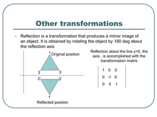
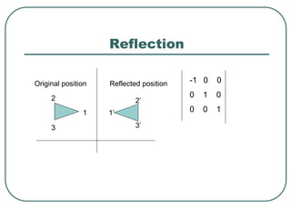
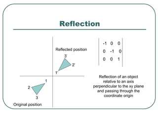
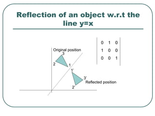
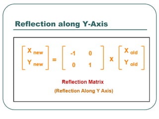
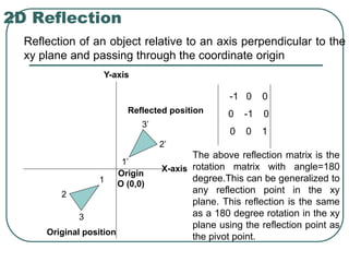
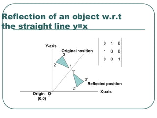
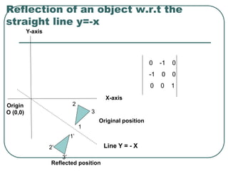
Reflections
Initial
Object
Reflection about x
y =  y
x
y
Reflection about
origin
x =  x
y =  y
Reflection about y
x =  x

37. Reflection along X-Axis

38. Reflection along Y-Axis

39. 2D Reflection
-1 0 0
0 -1 0
0 0 1
1’
2’
3’
3
2
1
Original position
Reflected position
Reflection of an object relative to an axis perpendicular to the
xy plane and passing through the coordinate origin
X-axis
Y-axis
Origin
O (0,0)
The above reflection matrix is the
rotation matrix with angle=180
degree.This can be generalized to
any reflection point in the xy
plane. This reflection is the same
as a 180 degree rotation in the xy
plane using the reflection point as
the pivot point.

40. Reflection of an object w.r.t
the straight line y=x
0 1 0
1 0 0
0 0 1
1’
3’
2’
3
2 1
Original position
Reflected position
X-axis
Y-axis
Origin O
(0,0)

41. Reflection of an object w.r.t the
straight line y=-x
0 -1 0
-1 0 0
0 0 1
1’
3’
2’
3
X-axis
1
Original position
Reflected position
2
Y-axis
Origin
O (0,0)
Line Y = - X

42. Problem-01:
 Given a triangle with coordinate points
A(3, 4), B(6, 4), C(5, 6). Apply the
reflection on the X axis and obtain the
new coordinates of the object.

43. Solution

44. Exercise
 Given a triangle with coordinate points
A(3, 4), B(6, 4), C(5, 6). Apply the
reflection on the Y axis and obtain the
new coordinates of the object.

45. Solution

46. 2D Shear
 Shear is a transformation that distorts the
shape of an object such that the transformed
shape appears as if the object were
composed of internal layers that had been
caused to slide over each other
 Two common shearing transformations are
those that shift coordinate x values and those
that shift y values

47. Shearing
 Shearing in X direction
 Shearing in Y direction
Let-
 Initial coordinates of the object O = (Xold, Yold)
 Shearing parameter towards X direction = Shx
 Shearing parameter towards Y direction = Shy
 New coordinates of the object O after shearing =
(Xnew, Ynew)

48. Shear
  
 
x x h y
y y
x
•A shear transformation in the x-direction (along x)
shifts the points in the x-direction proportional
to the y-coordinate.
•The y-coordinate of each point is unaffected.

49. 2D Shears
Original Data y Shear x Shear
1 0 0 1 shx 0
shy 1 0 0 1 0
0 0 1 0 0 1

50. Shearing Along X-axis

51. Shearing Along Y-axis

52. An X- direction Shear
(0,1) (1,1)
(1,0)
(0,0) (0,0) (1,0)
(2,1) (3,1)
For example, Shx=2

53. An Y- direction Shear
(0,1) (1,1)
(1,0)
(0,0) (0,0)
(0,1)
(1,3)
(1,2)
For example, Shy=2
X X
Y Y

54. Problem-01:
 Given a triangle with points (1, 1), (0, 0)
and (1, 0). Apply shear parameter 2 on X
axis and 2 on Y axis and find out the
new coordinates of the object.

56. 






 





 













 




















 












x
y
x
y
t
t
x
y
x
y
x
y
s
s
x
y
x
y
x
y
cos sin
sin cos
 
 
0
0
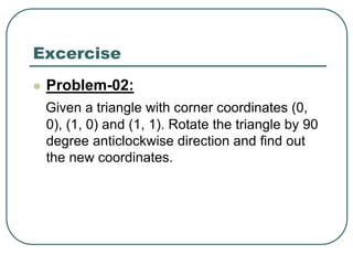
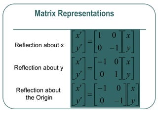
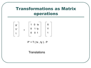
Translation
Rotation [Origin]
Scaling [Origin]
Matrix Representations

57. 

































































y
x
y
x
y
x
y
x
y
x
y
x
1
0
0
1
1
0
0
1
1
0
0
1
Reflection about x
Matrix Representations
Reflection about y
Reflection about
the Origin

58. [6]-58 RM










































y
x
h
y
x
y
x
h
y
x
1
0
1
1
0
1
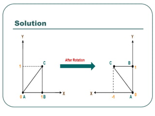
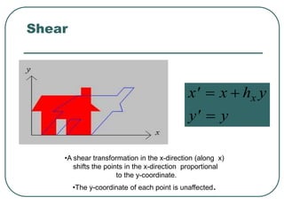
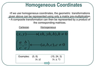
Shear along x
Matrix Representations
Shear along y

59. [6]-59 RM
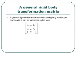
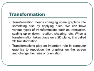
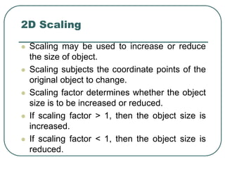
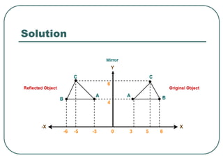
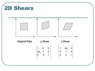
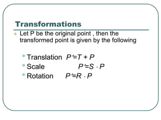
Homogeneous Coordinates
To obtain square matrices an additional row was added to the matrix
and an additional coordinate, the w-coordinate, was added to the
vector for a point. In this way a point in 2D space is expressed in
three-dimensional homogeneous coordinates.
This technique of representing a point in a space whose dimension is
one greater than that of the point is called homogeneous
representation. It provides a consistent, uniform way of handling affine
transformations.

60. Cartesian Homogeneous
0
),
,
,
(
,
0
),
,
,
(
)
,
(












c
c
b
a
c
b
c
a
h
h
yh
xh
y
x
Examples: (5, 8) (15, 24, 3)
(x, y) (x, y, 1)
Homogeneous Coordinates
•If we use homogeneous coordinates, the geometric transformations
given above can be represented using only a matrix pre-multiplication.
• A composite transformation can then be represented by a product of
the corresponding matrices.

61. Transformations
 Let P be the original point , then the
transformed point is given by the following
•Translation P=T + P
•Scale P=S  P
•Rotation P=R  P

62. 



































































































x
y
t
t
x
y
x
y
x
y
x
y
s
s
x
y
x
y
x
y
1
1 0
0 1
0 0 1 1
1
0
0
0 0 1 1
1
0 0
0 0
0 0 1 1
cos sin
sin cos
 
 
Translation
P’=TP
Rotation [O]
P’=RP
Scaling [O]
P’=SP
Basic Transformations
Homogeneous Coordinates

63. 






















1
]
[
1
y
x
T
y
x
If,
























1
]
[
1
1
y
x
T
y
x
then,
)
(
)
(
1
,
1
)
,
(
)
(
)
(
)
,
(
)
,
(
1
1
1
1
h
H
h
H
s
s
S
s
s
S
R
R
t
t
T
t
t
T
x
x
y
x
y
x
y
x
y
x






















Examples:
Inverse of Transformations

64. Transformations as Matrix
operations
X’
Y’
1
1 0 tx
0 1 ty
0 0 1
X
Y
1
P’ = T ( tx , ty ) . P
=
Translations

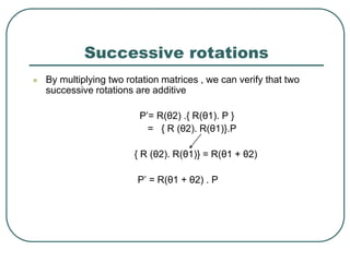
65. Successive translations
Successive translations are additive
P’= T(tx1, ty1) .[T(tx2, ty2)] P
= {T(tx1, ty1). T(tx2, ty2)}.P
T(tx1, ty1). T(tx2, ty2) = T(tx1+tx2 , ty1 + ty2)
1 0 tx1+tx2
0 1 ty1+ty2
0 0 1
1 0 tx1
0 1 ty1
0 0 1
1 0 tx2
0 1 ty2
0 0 1
=

66. Successive rotations
 By multiplying two rotation matrices , we can verify that two
successive rotations are additive
P’= R(θ2) .{ R(θ1). P }
= { R (θ2). R(θ1)}.P
{ R (θ2). R(θ1)} = R(θ1 + θ2)
P’ = R(θ1 + θ2) . P

67. Successive Scaling operations
Sx1.sx2 0 0
0 sy1sy2 0
0 0 1
sx1 0 0
0 sy1 0
0 0 1
sx2 0 0
0 sy2 0
0 0 1
=
S(sx2,sy2).S(sx1,sy1) = S(sx1.sx2 , sy1,sy2)
The resulting matrix in this case indicates that successive scaling
operations are multiplicative

68. General pivot point rotation
 Translate the object so that pivot-position is moved to the
coordinate origin
 Rotate the object about the coordinate origin
 Translate the object so that the pivot point is returned to its original
position
(xr,yr)
(a)
Original Position
of Object and
pivot point
(b)
Translation of
object so that
pivot point
(xr,yr)is at origin
(c)
Rotation was
about origin
(d)
Translation of the object
so that the pivot point is
returned to position
(xr,yr)

69. Thank You

70. General pivot point rotation
1 0 xr
0 1 yr
0 0 1
cosθ -sinθ 0
sinθ cosθ 0
0 0 1
1 0 -xr
0 1 -yr
0 0 1
=
cosθ -sinθ xr(1- cosθ)+ yr sinθ
sinθ cosθ yr(1- cosθ) - xr sinθ
0 0 1
Can also be expressed as T(xr,yr).R(θ).T(-xr,-yr) = R(xr,yr,θ)

71. General fixed point scaling
 Translate object so that the fixed point coincides with the
coordinate origin
 Scale the object with respect to the coordinate origin
 Use the inverse translation of step 1 to return the object to its
original position
(xf,yf)
(a)
Original Position
of Object and
Fixed point
(b)
Translation of
object so that
fixed point
(xf,yf)is at origin
(c)
scaling was
about origin
(d)
Translation of the object
so that the Fixed point
is returned to position
(xf,yf)

72. General pivot point Scaling
1 0 xf
0 1 yf
0 0 1
sx 0 0
0 sy 0
0 0 1
1 0 -xf
0 1 -yf
0 0 1
=
sx 0 xf(1- sx)
0 sy yf(1- sy)
0 0 1
Can also be expressed as T(xf,yf).S(sx,sy).T(-xf,-yf) = S(xf, yf, sx, sy)

73. Transformations Properties
 Concatenation properties
A.B.C = (A.B).C = A.(B.C)
Matrix products can be evaluated from left to right or from right
to left
 However they are not commutative
A.B ≠ B.A
 Hence one must be careful in order that the composite
transformation matrix is evaluated

74. Order of Transformations
 Reversing the order in which a sequence of transformations is
performed may effect the transformed position of an object.
 In (a) object is first translated , then rotated
 In (b) the object is rotated first and then translated
(a) (b)

75. General Composite
transformations
 A general 2D transformation representing a combination of translations,
rotations and scalings are expressed as,
 rsij represent multiplicative rotation-scaling terms , trsx and trsy are the
translational terms containing combinations of translations and scaling
parameters
X’
Y’
1
=
rsxx rsxy trsx
rsyx rsyy trsy
0 0 1
X
Y
1

76. Composite transformations
 For example , if an object is to be scaled and rotated about its
center coordinates (xc,yc) and then translated , the composite
transformation matrix looks like
 T(tx,ty). R(xc,yc,θ) . S(xc, yc, sx, sy)
=
sxcosθ -sysinθ xc(1-sxcosθ) + yc sy sinθ +tx
sxsin θ sycos θ yc(1-sycosθ) – xc sx sinθ + ty
0 0 1
Represents 9 multiplications and 6 additions

77. Composite Transformations
 The explicit calculation has only 4 multiplications and 4
additions
x’ = x.rsxx + y.r sxy + tr sx
y’ = x. rsyx + y. rsyy + tr sy
 The efficient implementation is to
• Formulate transformation matrices
• Concatenate transformation sequence
• Calculate transformed coordinates using the explicit
equation shown above

78. A general rigid body
transformation matrix
 A general rigid body transformation involving only translations
and rotations can be expressed in the form
rxx rxy trx
ryx ryy try
0 0 1

79. Other transformations
 Reflection is a transformation that produces a mirror image of
an object. It is obtained by rotating the object by 180 deg about
the reflection axis
1
2 3
3’
2’
1’
Original position
Reflected position
Reflection about the line y=0, the
axis , is accomplished with the
transformation matrix
1 0 0
0 -1 0
0 0 1

80. Reflection
-1 0 0
0 1 0
0 0 1
1’
3’
2’
3
2
1
Original position Reflected position

81. Reflection
-1 0 0
0 -1 0
0 0 1
1’
2’
3’
3
2
1
Original position
Reflected position
Reflection of an object
relative to an axis
perpendicular to the xy plane
and passing through the
coordinate origin

82. Reflection of an object w.r.t the
line y=x
0 1 0
1 0 0
0 0 1
1’
3’
2’
3
2 1
Original position
Reflected position

83. Shear Transformations
 Shear is a transformation that distorts the shape of an object
such that the transformed shape appears as if the object were
composed of internal layers that had been caused to slide over
each other
 Two common shearing transformations are those that shift
coordinate x values and those that shift y values
 An x direction shear relative to the x axis is produced with the
transformation matrix
1 shx 0
0 1 0
0 0 1
Which transforms coordinate positions as
X’ = x + shx.y y’ =y

84. Shear tranformations
Yref =-1
Yref =-1
(0,1) (1,1)
(1,0)
(0,0)
(1,1) (2,1)
(3/2,0)
(1/2,0)
We can generate x-direction shears relative to other referance lines with
1 shx -shx yref
0 1 0
0 0 1
With coordinate positions transformed as
X’= x + shx (y - yref) y’ = y

85. Shear transformation
A y-direction shear relative to the line x = xref is generated with the
transformation matrix
1 0 0
Shy 1 -shy.xref
0 0 1
This generates transformed coordinate
positions
X’ = x y’ = shy (x – xref) + y
(1,1)
(0,1)
(0,0) (1,0)
(1,2)
(1,1)
(0,1/2)
(0,3/2)
Xref = -1