Downloaded 39 times


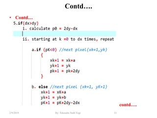


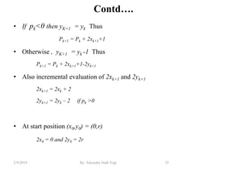
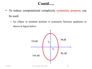
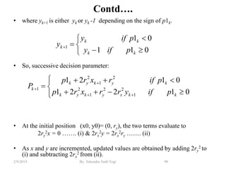
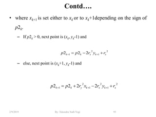
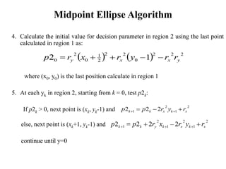
![Contd….
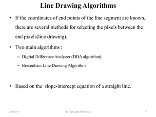
• Successive decision parameter at sampling position xk+1+1
=xk+2 is:
54By: Tekendra Nath Yogi2/9/2019
1)()()1(2
)
2
1
(]1)1[(
)
2
1
,1(
1
22
11
22
1
2
111
kkkkkkk
kk
kkcirclek
yyyyxpp
ryx
yxfp](https://image.slidesharecdn.com/unit1-190209042002/85/B-SC-CSIT-Computer-Graphics-Unit1-2-By-Tekendra-Nath-Yogi-54-320.jpg)
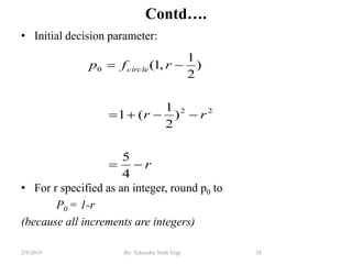


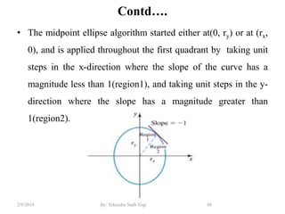
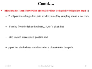
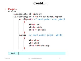
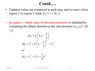
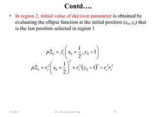
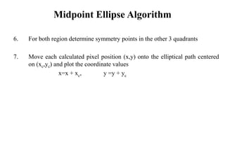
![Contd….
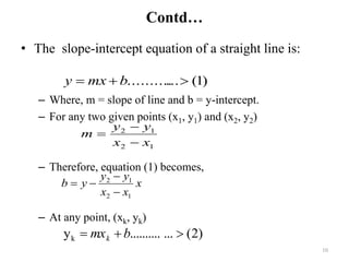
• At the next sampling position (xk+1 + 1 = xk + 2), the decision
parameter for region 1 is evaluated as
where yk+1 is either yk or yk -1 depending on the sign of p1k.
89By: Tekendra Nath Yogi2/9/2019
22
1
222
1
22
2
1
222
2
1
111
2
1
2
1
)1(211
2
1
]1)1[(
,11
kkxykykk
yxkxky
kkek
yyrrxrpp
or
rryrxr
yxfp](https://image.slidesharecdn.com/unit1-190209042002/85/B-SC-CSIT-Computer-Graphics-Unit1-2-By-Tekendra-Nath-Yogi-89-320.jpg)
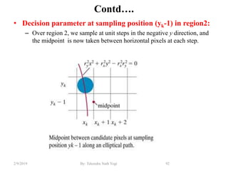
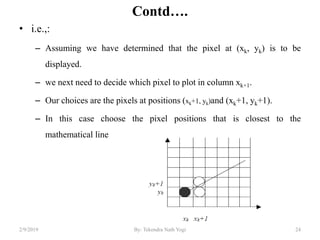
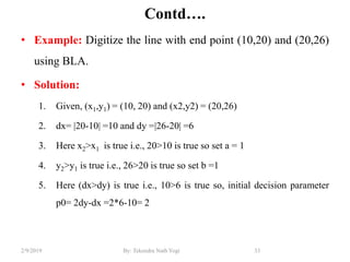
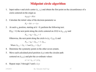
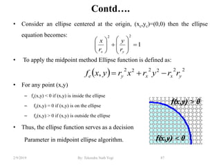
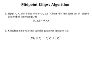
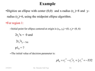
![Contd….
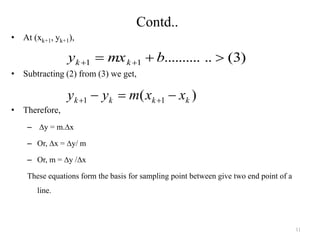
• At the next sampling position (yk+1 - 1 = yk - 2), the decision
parameter for region 2 is evaluated as:
• where xk+1 is set either to xk or to xk+1depending on the sign of
p2k.
94By: Tekendra Nath Yogi2/9/2019
22
1
222
1
2222
2
1
2
12
1
11
2
1
2
1
)1(222
]1)1[(
2
1
1,2
kkyxkxkk
yxkxky
kkek
xxrryrpp
or
rryrxr
yxfp](https://image.slidesharecdn.com/unit1-190209042002/85/B-SC-CSIT-Computer-Graphics-Unit1-2-By-Tekendra-Nath-Yogi-94-320.jpg)


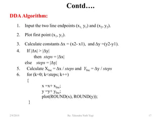
1. The document discusses raster graphics and algorithms for drawing basic 2D primitives like points, lines, circles, and polygons. 2. It describes two common line drawing algorithms - the Digital Differential Analyzer (DDA) algorithm and Bresenham's line algorithm. 3. The DDA algorithm draws lines by calculating pixel positions using the slope of the line, while Bresenham's algorithm uses only integer calculations to find the next pixel position along the line.