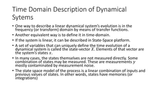
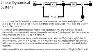
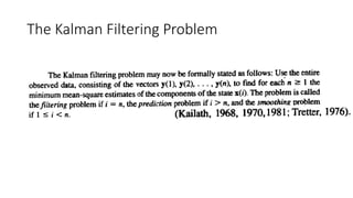
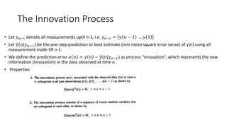
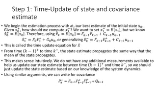
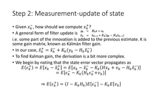
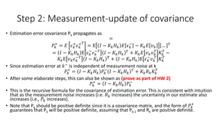
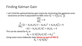
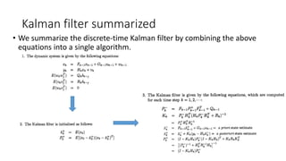
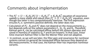
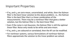
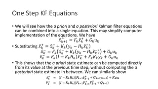
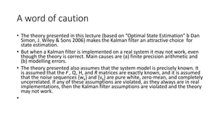
This document covers Kalman filters, emphasizing their optimal and recursive nature, discrete-time implementation, and state-space representation. It details the processes involved in state estimation, including time and measurement updates, innovation, and covariance propagation, alongside derivations and practical examples. The presentation also highlights the limitations and assumptions of Kalman filters when applied to real-world systems, including modeling errors and finite precision arithmetic.

1. Av-738
Adaptive Filter Theory
Lecture 4- Optimum Filtering
[Kalman Filters]
Dr. Bilal A. Siddiqui
Air University (PAC Campus)
Spring 2018

2. Kalman Filters
• Kalman filter is both an optimal and recursive (adaptive filter)
• It has a unique mathematical formulation (i.e. state space concepts)
• It is solved recursively. It is updated using previous state estimates and
new data (innovation), therefore no need for storage.
• It is mostly implemented in the discrete form, and easily implementable
on digital computers
• It gives a unifying framework for RLS filters.
• Developed by Rudolf Kalman in 1969 []

3. Time Domain Description of Dynamical
Sytems
• One way to describe a linear dynamical system’s evolution is in the
frequency (or transform) domain by means of transfer functions.
• Another equivalent way is to define it in time-domain.
• If the system is linear, it can be described in State-Space platform.
• A set of variables that can uniquely define the time evolution of a
dynamical system is called the state-vector 𝑋. Elements of that vector are
the system’s states 𝑥.
• In many cases, the states themselves are not measured directly. Some
combination of states may be measured. These are measurements 𝑦
mostly contaminated by measurement noise.
• The state space model of the process is a linear combination of inputs and
previous values of states. In other words, states have memories (or
integrations)

4. Linear Dynamical
System
• v1 is process “noise” which is a measure of how inaccurate our linear model given by
𝑥 𝑛 + 1 = 𝐹 𝑛 + 1, 𝑛 𝑥 𝑛 + 𝑣1(𝑛) is. If there are M states, 𝑂 𝐹 = 𝑀 × 𝑀 and 𝑂 𝑥 =
𝑀 × 1, 𝑂 𝑣 = 𝑀 × 1
• F is known as the state transition matrix relating states at n+1 and n. Process noise is
measured as zero mean white noise (its correlation matrix Q1 is diagonal). Let the system be
time-invariant. The 𝐹 𝑛 + 1, 𝑛 = 𝐹 for all n.
• Measured quantities are linear combinations of states 𝑦 𝑛 = 𝐶 𝑛 𝑥 𝑛 + 𝑣2 𝑛 . For N
measurements, 𝑂 𝑦 = 𝑁 × 1, 𝑂 𝐶 = N × 𝑀 and 𝑣2 is a Nx1 measurement noise vector,
which may represent sensor noise and linearization errors. Its correlation matrix Q2 is also
diagonal.
• It is assumed that process and measurement noises are uncorrelated. 𝐸 𝑣1 𝑛 𝑣2
𝐻
(𝑛) = 0

5. The Kalman Filtering Problem

6. The Innovation Process
• Let 𝑦 𝑛−1 denote all measurements uptil n-1, i.e. 𝑦 𝑛−1 = 𝑦 𝑛 − 1 … 𝑦 1
• Let 𝑦(𝑛|𝑦 𝑛−1) be the one-step prediction or best estimate (min mean square error sense) of y(n) using all
measurement made till n-1.
• We define the prediction error 𝛼 𝑛 = 𝑦 𝑛 − 𝑦(𝑛|𝑦 𝑛−1) as process “innovation”, which represents the new
information (innovation) in the data observed at time n.
• Properties:

7. Innovation Propagation
• Suppose we have the more generic system 𝑥 𝑘 = 𝐹𝑥 𝑘 + 𝑣1(𝑛), then we can write a recursive relation
𝑥 𝑛 + 1 = 𝐹 𝑛
𝑥 0 +
𝑖=0
𝑛−1
𝐹 𝑛−1−𝑖
𝑣1 𝑖
• multiplying v2(n) and taking expectation
𝐸 𝑥 𝑛 + 1 𝑣2
𝐻
𝑛 = 𝐹𝐸 𝑥 0 𝑣2
𝐻
𝑛 + 𝐸
𝑖=0
𝑛−1
𝐹 𝑛−1−𝑖
𝑣1 𝑖 𝑣2
𝐻
𝑛
• Since noise v2 is uncorrelated with initial state x(0) and noise v1 this means 𝐸 𝑥 𝑘 𝑣2
𝐻
𝑛 for 0 ≤ 𝑘 ≤ 𝑛.
• Since 𝑦 𝑛 = 𝐶𝑥 𝑛 + 𝑣2 𝑛 , we can also prove that 𝐸 𝑦 𝑘 𝑣2
𝐻
𝑛 = 0 for 0 ≤ 𝑘 ≤ 𝑛 − 1 , i.e. v2 is orthogonal to past measurements.
• Therefore, 𝑦 𝑛 𝑦 𝑛−1 = C 𝑥(𝑛|𝑦 𝑛−1) as v2 cannot be predicted using past measurements.
• Therefore we can write innovations as 𝛼 𝑛 = 𝑦 𝑛 − C 𝑥(𝑛|𝑦 𝑛−1)
• Substitute measurement equation,
𝛼 𝑛 = 𝐶𝑥 𝑛 + 𝑣2 𝑛 − C 𝑥 𝑛 𝑦 𝑛−1 = 𝐶𝜖 𝑛, 𝑛 − 1 + 𝑣2(𝑛)
where 𝜖 𝑛, 𝑛 − 1 = 𝑥 𝑛 − 𝑥 𝑛 𝑦 𝑛−1 is the predicted state-error vector at n using the measurements till n-1
We can prove that 𝜖 𝑛, 𝑛 − 1 is orthogonal to v1 and v2 for for all times less than n.

8. A more generic model
• Suppose we have a more generalized process model of a discrete-
time linear system
𝑥 𝑘 = 𝐹𝑘−1 𝑥 𝑘−1 + 𝐺 𝑘−1 𝑢 𝑘−1 + 𝑤 𝑘−1
where uk is a known and deterministic input and wk is Gaussian zero-
mean white noise with covariance Qk.
• How does the mean of the state xk change with time?
𝑥 𝑘 = 𝐸 𝑥 𝑘 = 𝐹𝑘−1 𝑥 𝑘−1 + 𝐺 𝑘−1 𝑢 𝑘−1
• Now, how does the covariance of xk change with time?

9. Covariance Propagation
• Since
• Note that innovation or state error 𝜖 𝑘 = 𝑥 𝑘 − 𝑥 𝑘 is uncorrelated with noise
wk-1 (or process noise at k-1, as we said earlier)
• This means the state covariance matrix propagates as
This is called the discrete-time Lyapunov equation or Stein equation. Also note that since x0 and wi are
Gaussian 𝑥 𝑘 = 𝑁( 𝑥 𝑘, 𝑃𝑘)

10. Example (Predator + Prey)

11. Homework 2 (a)
• Simulate this model using Matlab
• But we could also have found the steady states and covariances
directly. Prove that the expression for steady states analytically are:

12. Derivation of the Kalman Filter
Our goal is to estimate the state xk based on our knowledge of the system
dynamics and the availability of the noisy measurements yk. The amount of
information that is available to us for our state estimate varies depending on
the particular problem that we are trying to solve.

13. Posteriors and Priots
• If we have all of the measurements up to and including time k available for use in
our estimate of xk, then we can form an a posteriori estimate, which we denote
as 𝑥 𝑘
+
• If we have all of the measurements before (but not including) time k available for
use in our estimate of xk , then we can form an a postiori estimate, which we
denote as 𝑥 𝑘
−

14. Process of Estimation
• After we process the measurement at time (k-1), we have an
estimate Of xk−1(denoted xk−1
+
) and the covariance of that estimate
(denoted Pk−1
+
).
• When time k arrives, before we process the measurement at time k,
we compute an estimate of 𝑥 𝑘(denoted 𝑥 𝑘
−
) and
the covariance of that estimate (denoted Pk
−
).
• Then we process the measurement at time k to refine our estimate of
𝑥 𝑘. The resulting estimate is denoted 𝑥 𝑘
−
, with covariance Pk
+
.

15. Step 1: Time-Update of state and covariance
estimate
• We begin the estimation process with at, our best estimate of the initial state x0.
Given 𝑥0
+
, how should we compute 𝑥1
−
? We want to set 𝑥1
−
= 𝐸 𝑥1 , but we know
𝑥0
+
= 𝐸 𝑥0 . Therefore, using 𝑥 𝑘 = 𝐸 𝑥 𝑘 = 𝐹𝑘−1 𝑥 𝑘−1 + 𝐺 𝑘−1 𝑢 𝑘−1
𝑥1
−
= 𝐹0 𝑥0
+
+ 𝐺0 𝑢0, or generalizing 𝑥 𝑘
−
= 𝐹𝑘−1 𝑥 𝑘−1
+
+ 𝐺 𝑘−1 𝑢 𝑘−1
• This is called the time update equation for 𝑥
• From time 𝑘 − 1 +
to time 𝑘−
, the state estimate propagates the same way that the
mean of the state propagates.
• This makes sense intuitively. We do not have any additional measurements available to
help us update our state estimate between time 𝑘 − 1 +
and time 𝑘−
, so we should
just update the state estimate based on our knowledge of the system dynamics.
• Using similar arguments, we can write for covariance

16. Step 2: Measurement-update of state
• Given 𝑥 𝑘
−
, how should we compute 𝑥 𝑘
+
?
• A general form of filter update is
i.e. some part of the innovation is added to the previous estimate. K is
some gain matrix, known as Kàlmàn filter gain.
• In our case, 𝑥 𝑘
+
= 𝑥 𝑘
−
+ 𝐾𝑘 𝑦 𝑘 − 𝐻 𝑘 𝑥 𝑘
−
• To find Kalman gain, the derivation is a bit more complex.
• We begin by noting that the state error vector propagates as
𝐸 𝜖 𝑘
+
= 𝐸 𝑥 𝑘 − 𝑥 𝑘
+
= 𝐸 𝑥 𝑘 − 𝑥 𝑘
−
− 𝐾𝑘 𝐻𝑥 𝑘 + 𝑣 𝑘 − 𝐻 𝑘 𝑥 𝑘
−
= 𝐸 𝜖 𝑘
−
− 𝐾𝑘(𝐻 𝑘 𝜖 𝑘
−
+𝑣 𝑘)
⇒ 𝐸 𝜖 𝑘
+
= 𝐼 − 𝐾𝑘 𝐻 𝑘 𝐸 𝜖 𝑘
−
− 𝐾𝑘 𝐸 𝑣 𝑘

17. Step 2: Measurement-update of covariance
• Estimation error covariance Pk propagates as
=
𝑃𝑘
+
= 𝐸 𝜖 𝑘
+
𝜖 𝑘
+ 𝑇
= E 𝐼 − 𝐾𝑘 𝐻 𝑘 𝐸 𝜖 𝑘
−
− 𝐾𝑘 𝐸 𝑣 𝑘 … 𝑇
= 𝐼 − 𝐾𝑘 𝐻 𝑘 E 𝜖 𝑘
−
𝜖 𝑘
−𝑇
𝐼 − 𝐾𝑘 𝐻 𝑘
𝑇
+ 𝐾𝑘 𝐸 𝑣 𝑘 𝑣 𝑘
𝑇
𝐾𝑘
𝑇
−
𝐾𝑘E 𝑣 𝑘 𝜖 𝑘
−𝑇
𝐼 − 𝐾𝑘 𝐻 𝑘
T + 𝐼 − 𝐾𝑘 𝐻 𝑘 E 𝜖 𝑘
−
𝑣 𝑘
𝑇
𝐾𝑘
𝑇
• Since estimation error at 𝑘−
is independent of measurement noise at k
𝑃𝑘
+
= 𝐼 − 𝐾𝑘 𝐻 𝑘 𝑃𝑘
−
𝐼 − 𝐾𝑘 𝐻 𝑘
𝑇 + 𝐾𝑘 𝑅 𝑘 𝐾𝑘
𝑇
• After some elaborate steps, this can also be shown as (prove as part of HW 2)
𝑃𝑘
+
= 𝐼 − 𝐾𝑘 𝐻 𝑘 𝑃𝑘
−
• This is the recursive formula for the covariance of estimation error. This is consistent with intuition
that as the measurement noise increases (i.e. 𝑅 𝑘 increases) the uncertainty in our estimate also
increases (i.e., 𝑃𝑘 increases).
• Note that Pk should be positive definite since it is a covariance matrix, and the form of 𝑃𝑘
+
guarantees that Pk will be positive definite, assuming that Pk-1 and Rk are positive definite.

18. Finding Kalman Gain
• Let’s find the optimal Kalman gain matrix by minimizing the posterior error
covariance at time k (equivalent to MSE since 𝑃𝑘
+
= 𝐸 𝜖 𝑘
+
𝜖 𝑘
+ 𝑇
).
𝜕𝑃𝑘
+
𝜕𝐾𝑘
= 0
𝜕
𝜕𝐾𝑘
𝐼 − 𝐾𝑘 𝐻 𝑘 𝑃𝑘
−
𝐼 − 𝐾𝑘 𝐻 𝑘
𝑇 + 𝐾𝑘 𝑅 𝑘 𝐾𝑘
𝑇
= 0
−2 𝐼 − 𝐾𝑘 𝐻 𝑘 𝑃𝑘
−
𝐻 𝑘
𝑇
+ 2𝐾𝑘 𝑅 𝑘 = 0
This can be solved for KK as
𝐾𝑘 = 𝑃𝑘
−
𝐻 𝑘
𝑇
𝐻 𝑘 𝑃𝑘
−
𝐻 𝑘
𝑇
+ 𝑅 𝑘
−1
Using some more elaborate steps (prove as part of HW 2)
𝐾𝑘 = Pk
+
Hk
T
Rk
−1

19. Kalman filter summarized
• We summarize the discrete-time Kalman filter by combining the above
equations into a single algorithm.

20. Comments about implementation
• The 𝑃𝑘
+
= 𝐼 − 𝐾𝑘 𝐻 𝑘 𝑃𝑘
−
𝐼 − 𝐾𝑘 𝐻 𝑘
𝑇
+ 𝐾𝑘 𝑅 𝑘 𝐾𝑘
𝑇
equation of covariance
update is more stable and robust than 𝑃𝑘
+
= 𝐼 − 𝐾𝑘 𝐻 𝑘 𝑃𝑘
−
equation, even
though the latter is less computationally intensive. The first expression
ensures Pk is symmetric positive definite, the latter does not.
• Calculation of 𝑃𝑘
−
, 𝐾𝑘and 𝑃𝑘
+
does not depend on the measurements yk ,
but depends only on the system parameters Fk, Hk, Qk and Rk. Therefore,
Kalman gain Kk can be calculated offline before the system operates and
saved in memory (if statistics Q, F and R are known). In that case, linear
time-invariant Kalman filter is like the Weiner filter and not adaptive.
• In contrast, as we will see later, the filter gain and covariance for nonlinear
systems cannot (in general) be computed offline because they depend on
the measurements. In that case, the Kalman filter has important nonlinear
variants.

21. Important Properties
• If wk and vk are zero-mean, uncorrelated, and white, then the Kalman
filter is the best linear solution to the above problem, i.e., the Kalman
filter is the best filter that is a linear combination of the
measurements. There may be a nonlinear filter that gives a better
solution, but the Kalman filter is the best linear filter.
• Even if the noise is not Gaussian, the Kalman filter is still the optimal
linear filter. Noise only needs to be white and zero-mean.
• If wk and vk are coloured or correlated, then the KF can be modified.
• For nonlinear systems, various formulations of nonlinear Kalman
filters approximate the solution to the linear problem we solved.

22. One Step KF Equations
• We will see how the a priori and a posteriori Kalman filter equations
can be combined into a single equation. This may simplify computer
implementation of the equations. We have
𝑥 𝑘+1
−
= 𝐹𝑘 𝑥 𝑘
+
+ 𝐺 𝑘 𝑢 𝑘
• Substituting 𝑥 𝑘
+
= 𝑥 𝑘
−
+ 𝐾𝑘 𝑦 𝑘 − 𝐻 𝑘 𝑥 𝑘
−
𝑥 𝑘
−
= 𝐹𝑘 𝑥 𝑘
−
+ 𝐾𝑘 𝑦 𝑘 − 𝐻 𝑘 𝑥 𝑘
−
+ 𝐺 𝑘 𝑢 𝑘
𝑥 𝑘
−
= 𝐹𝑘 𝐼 − 𝐾𝑘 𝐻 𝑘 𝑥 𝑘
−
+ 𝐹𝑘 𝐾𝑘 𝑦 𝑘 + 𝐺 𝑘 𝑢 𝑘
• This shows that the a priori state estimate can be computed directly
from its value at the previous time step, without computing the a
posteriori state estimate in between. We can similarly show

23. Example
• Suppose we have a noise-free with position r , velocity v, and
constant acceleration a.

24. Solution

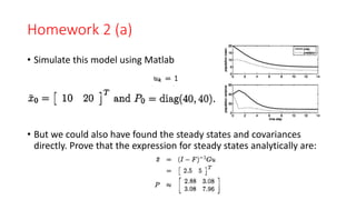
25. Simulation
%%
clc;clear all;close;
%Kalman filter for position measurement
%AV-738 Spr 18, Dr. Bilal A. Siddiqui
T=5;
R=30^2;
a=0.01;
F=[1 T T^2/2 %position
0 1 T %velocity
0 0 1]; %acceleration
G=0;
H=[0 0 1];% only position being measured
w=0;%process noise
x(:,1)=[0 0 a]';%initial value of state vector
x_post(:,1)=[0 0 0]';%initial estimate of state
vector
P_post(:,:,1)=1E5*eye(3);%initial estimate of error
covariance
for k=2:60
%calculate a priori covariance estimate
P_prior(:,:,k)=F*P_post(:,:,k-1)*F';
%calculate Kalman gain
K(:,:,k)=P_prior(:,:,k)*H'*(H*P_prior(:,:,k)*H'+R)^-1;
%calculate a priori estimate of state
x_prior(:,k)=F*x(:,k-1);
%system evolution
x(:,k)=F*x(:,k-1);%take measurement
y(k)=H*x(:,k)+sqrt(R)*randn;
%calculate innovation
innov(k)=y(k)-H*x_prior(:,k);
%calculate a posteriori estimate of state
x_post(:,k)=x_prior(:,k)+K(:,:,k)*innov(k);
%calculate a posteriori estimate of covariance
P_post(:,:,k)=(eye(3)- ...
K(:,:,k)*H)*P_prior(:,:,k)*+(eye(3)-K(:,:,k)*H)'+...
K(:,:,k)*R*K(:,:,k)';
end

26. Results

27. Homework 2 (c)
• First of all, we were able to reduce estimation error below the
measurement noise floor. How was that possible?
• Also, if we start measuring the acceleration directly (use a 1-g noise,
i.e.R=1) instead of the position, we will get a good estimate still, but the
error covariance will keep increasing. Why?
• In practical terms, if we inject position measurements at a slower rate,
what will happen to the error covariance, if we were taking accelerometer
measurements at a higher rate?
• Simulate the error covariance if we measure accelerometer at every
sampling instant, but receive GPS position with noise variance of 10 after
every five sampling instants.
• Comment your answer and analyze the results.

28. A word of caution
• The theory presented in this lecture (based on “Optimal State Estimation” b Dan
Simon, J. Wiley & Sons 2006) makes the Kalman filter an attractive choice for
state estimation.
• But when a Kalman filter is implemented on a real system it may not work, even
though the theory is correct. Main causes are (a) finite precision arithmetic and
(b) modelling errors.
• The theory presented also assumes that the system model is precisely known. It
is assumed that the F , Q, H, and R matrices are exactly known, and it is assumed
that the noise sequences {wk} and {vk} are pure white, zero-mean, and completely
uncorrelated. If any of these assumptions are violated, as they always are in real
implementations, then the Kalman filter assumptions are violated and the theory
may not work.
•

29. Some Remedies