The Wiener filter is a signal processing filter that reduces noise in a signal. It was proposed by Norbert Wiener in 1940 and published in 1949. The Wiener filter takes a statistical approach to minimize the mean square error between an original noiseless signal and the estimated signal by assuming knowledge of the spectral properties of the original signal and noise. It is commonly used for noise reduction and image deblurring. The Wiener filter implementation is available in Matlab and Python and its performance depends on the noise parameters used.

1. WIENER FILTER

2. INTRODUCTION
• The Wiener filter was proposed by Norbert Wiener in
1940.
• It was published in 1949
• Its purpose is to reduce the amount of a noise in a
signal.
• This is done by comparing the received signal with a
estimation of a desired noiseless signal.
• Wiener filter is not an adaptive filter as it assumes
input to be stationery.

3. DESCRIPTION
• It takes a statistical approach to solve its goal
• Goal of the filter is to remove the noise from a signal
• Before implementation of the filter it is assumed that
the user knows the spectral properties of the original
signal and noise.
• Spectral properties like the power functions for both
the original signal and noise.
• And the resultant signal required is as close to the
original signal

4. DESCRIPTION
• Signal and noise are both linear stochastic
processes with known spectral properties.
• The aim of the process is to have minimum mean-
square error
• That is, the difference between the original signal
and the new signal should be as less as possible.

5. Important Equations
• Considering we need to design a wiener filter in
frequency domain as W(u,v)
• Restored image will be given as;
Xn(u,v) = W(u,v).Y(u,v)
• Where Y(u,v) is the received signal and Xn(u,v) is the
restored image

6. Considering images and noise as random variables, the
ˆ
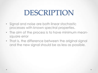
Important Equations
is to find an estimate f of the uncorrupted image f su
mean square error between them is minimized.
• We choose The error measure is given by
W(k,l) to minimize:
e 2 = E { (f − f )2 }
ˆ
Obtained from [1]
where E {i} is the expected value of the argument.
• Where the equation represents the mean square
error.
By assuming that
• The wiener filter can be represented by the
equation: 1. the noise and the image are uncorrelated;
2. one or the other has zero mean;
3. the intensity levels in the estimate are a linear fu
the levels in the degraded image.

7. Important Equations
• Obtained from [1]

8. Important Equations
• H(u,v) = degradation function
• |H(u,v)|^2 = H*(u,v)H(u,v)
• H*(u,v) = complex conjugate of H(u,v)
• Sn(u,v) = |N(u,v)|^2 power spectrum of noise
• Sf(u,v) = |F(u,v)|^2 power spectrum of
undegraded image
. G(u,v) is the transform of the degraded image.

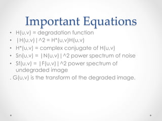
9. The Wiener filter does not have the same problem as the invers
filter with zeros in the degradation function, unless the entire
denominator is zero for the same value(s) of u and v .
Important Equations
If the noise is zero, then the Wiener filter reduces to the invers
filter.
• The signal to noise ration can be approximated
using One of the most important measures is the signal-to-noise ratio
the following equation:
approximated using frequency domain quantities such as
M −1 N −1
∑∑ F (u, v ) 2
u =0 v =0
SNR = M −1 N −1
(5.8-3)
∑∑ N (u, v ) 2
u =0 v =0
Obtained from [1]
• Low noise gives high SNR and High noise gives Low
SNR. The value is a good metric used in
characterizing the performance of restoration
algorithm

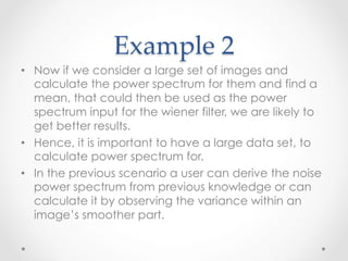
10. The mean square error given in statistical form in (5.8-1) can be
Important Equations
approximated also in terms a summation involving the original
and restored images:Image Processing (Fall Term, 2011-12) Page 291
• The MSE in statistical form can be calculated as:
ACS-7205-001 Digital
M −1 N −1
1
The mean square error given in statistical form in (5.8-1) can be
2
MSE =
and restored images:∑ ∑  f (x, y) − fˆ(x, y)
approximated also in terms a summation involving the original
MN x =0 y =0 M −1 N −1
(5.8-4)
1  f (x , y ) − f (x , y )  2
MSE = ∑ ∑
MN x = 0 y = 0 
Obtained from [1]
ˆ

 (5.8-4)
• If restored signal isthe restored image asbe signal and the difference
If one considers considered to signal and can define a
If one considers the restored image to be signal and the difference
difference between the thespatial domain noise, we
between this image and restored to be degraded as
original and
signal-to-noise ratio inthe original to be noise, we can define a
between this we can the
the noise, then
image and obtain SNR in spatial domain
as
signal-to-noise ratio in the∑ ∑ domain as
spatial fˆ(x, y)
M −1 N −1
2
x =0 y =0
SNR = M −1 N −1
2 (5.8-5)
∑ M −1 N −1 x, y ) − f (x, y ) 
∑ f( ˆ
x =0 y =0
ˆ ∑ ∑ f (x, y)
Obtained from ˆ
[1] 2
The closer f and f are, the larger this ratio will be.
x =0 y =0
SNR = 2
If we are dealing with white noise, the spectrum N (u, v ) is a
M −1 N −1

11. ∑ ∑  f (x, y) − f (x, y) 
x =0 y =0
Important Equations
The closer f and fˆ are, the larger this ratio will be.
N (u, v) 2 is a
• But it isare dealing withhard noise, the spectrum power
If we sometimes white to estimate the
spectrumwhich simplifies things considerably.image or the
constant, of either the un-degraded However,
noise., v ) 2
F (u is usually unknown.
• In that case we assume a constant K, that is then
added to allis used frequently when these quantities are not
An approach terms of H|(u,v)|^2
• The new equation in that case becomes:
known or cannot be estimated:
 1 H (u, v) 2 
ˆ
F (u, v) =   G(u, v)
 H (u, v) H (u, v) + K 
2 (5.8-6)
 
Obtained from [1]
where K is a specified constant that is added to all terms of
H (u, v) 2 .

12. Working Example 1
ACS-7205-001 Digital Image Processing (Fall Term, 2011-12)
7205-001 Digital Image Processing (Fall Term, 2011-12)
Page 293
Page 293
ample 5.13:apply Further comparisons of Wienerof images 293
• We 5.13: the filter to the following set filtering
Example Further comparisons of Wiener filtering
205-001 Digital Image Processing (Fall Term, 2011-12) Page
ACS-7205-001 Digital Image Processing (Fall Term, 2011-12) Page 2
mple 5.13: Further comparisons of Wiener filtering
Example 5.13: Further comparisons of Wiener filtering
1 obtained from [1] 2 Obtained from [1]
• We reduce the noise variance (noise power):
3 obtained from[1] 4 obtained from [1]

13. Working Example 1
• We decrease the noise variance even further:
5 obtained from [1] 6 obtained from [1]
• As we can see A wiener filter does a very good job
at deblurring of an image and reducing the noise.

14. Example 2
• The problem is to estimate the power spectrum of
noise and even more difficult is to estimate the
power spectrum of the image.
• We know that most of the images have similar
power spectrum.
• We take two images and calculate their individual
power spectrum
• The images derived are obtained from [2]

15. Example 2
Obtained from [2]

16. Example 2
• We calculate the power spectrum of each image:
Obtained from [2]

17. Example 2
• If we restore the cameraman image using its own
power spectrum, the image will look like this:
Obtained from [2]

18. Example 2
• But we use the power spectrum obtained from the
house image, the restored image will look like this:
Obtained from [2]

19. Example 2
• Now if we consider a large set of images and
calculate the power spectrum for them and find a
mean, that could then be used as the power
spectrum input for the wiener filter, we are likely to
get better results.
• Hence, it is important to have a large data set, to
calculate power spectrum for.
• In the previous scenario a user can derive the noise
power spectrum from previous knowledge or can
calculate it by observing the variance within an
image’s smoother part.

20. How to use Wiener filter?
• Implementation of wiener filter are available both in
Matlab and Python.
• These implementations can be used to perform
analysis on images.

21. Conclusion
• Wiener filter is an excellent filter when it comes to
noise reduction or deblluring of images.
• A user can test the performance of a wiener filter
for different parameters to get the desired results.
• It is also used in steganography processes.
• It considers both the degradation function and
noise as part of analysis of an image.

22. References
• [1] R. Gonzalez and W. RE, Digital Image
Processing, Third Edit. Pearson Prentice Hall, 2008,
pp. 352–357.
• [2] S. Eddins, “Matlab Central Steve on Image
Processing.” [Online]. Available: http://
blogs.mathworks.com/steve/2007/11/02/image-
deblurring-wiener-filter/. [Accessed: 25-Aug-2012].