MOFT Tutorials
Multi Object Filtering Multi Target Tracking
Kalman Filtering and Kalman Filters
Optimal Filtering
▪ methodology used for estimating the state of a time varying system,
observed through noisy measurements
▪ state refers to the physical state
▪ described by dynamic variables, such as position, velocity and
acceleration of a moving object
▪ noise in the measurements means a certain degree of uncertainty
▪ dynamic system evolves as a function of time, cannot be modelled
entirely deterministically
▪ noise in the dynamics of system, process noise,
Kalman Filtering and Kalman Filters
▪ filtering means the process of filtering out the noise in the
measurements
▪ and providing an optimal estimate for the state given the observed
measurements and the assumptions made about the dynamic system
Kalman Filtering and Kalman Filters
Discrete-Time State Space Models
▪ models where the states are defined on discrete time instances.
▪ defined recursively in terms of distributions
𝐱 𝑘~𝑝 𝐱 𝑘|𝐱 𝑘−1
𝐲 𝑘~𝑝 𝐲 𝑘|𝐱 𝑘
Kalman Filtering and Kalman Filters
▪ 𝐱 𝑘 ∈ ℝ 𝒏 is the state of the target on time step 𝑘, which can be, for
example, the position, the velocity or the acceleration of the target.
▪ 𝐲 𝑘 ∈ ℝ 𝒎 is the measurement on time step 𝑘, which can be, for
example, position of the target, distance to the target or the relative
angle between the target and the sensor.
Kalman Filtering and Kalman Filters
▪ 𝑝 𝐱 𝑘|𝐱 𝑘−1 is the dynamic model which characterizes the dynamic
behavior of the system
▪ usually the model is a probability density (continuous state), but it can
also be a counting measure (discrete state), or a combination of
them, if the state is both continuous and discrete.
▪ 𝑝 𝐲 𝑘|𝐱 𝑘 is the model for measurements, describes how the
measurements are distributed given the state.
▪ model characterizes how the dynamic model is perceived by the
observers
Kalman Filtering and Kalman Filters
▪ system defined this way has so called Markov-property,
▪ state 𝐱 𝑘 given 𝐱 𝑘−1 is independent from the history of states and
measurements,
▪ expressed as;
𝑝 𝐱 𝑘|𝐱1:𝑘−1, 𝐲1:𝑘−1 = 𝑝 𝐱 𝑘|𝐱 𝑘−1
𝑝 𝐱 𝑘−1|𝐱 𝑘:𝑇, 𝐲 𝑘:𝑇 = 𝑝 𝐱 𝑘−1|𝐱 𝑘
▪ measurement 𝐲 𝑘 is independent from the histories of measurements
and states,
▪ expressed with equality
𝑝 𝐲 𝑘|𝐱1:𝑘, 𝐲1:𝑘−1 = 𝑝 𝐲 𝑘|𝐱 𝑘
Kalman Filtering and Kalman Filters
General Dynamic Model and Measurement Model
Kalman Filtering and Kalman Filters
General Dynamic Model and Measurement Model
Kalman Filtering and Kalman Filters
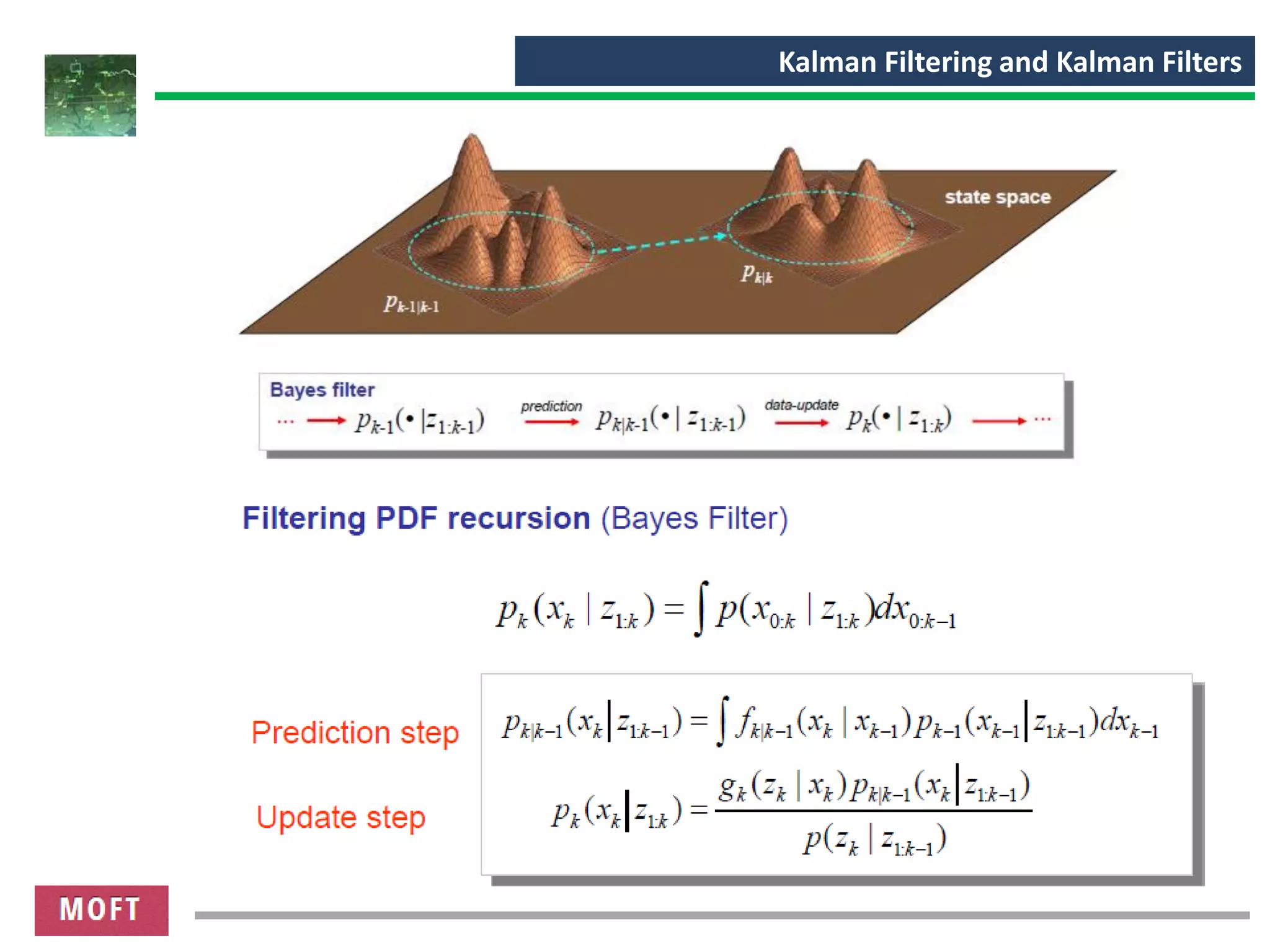
▪ problem - predicting and estimating dynamic system’s state given the
measurements obtained so far
▪ predictive distribution for the state at the next time step
𝑝 𝐱 𝑘|𝐲1:𝑘−1
▪ and marginal posterior distribution for the state at the current time
step
𝑝 𝐱 𝑘|𝐲1:𝑘
Kalman Filtering and Kalman Filters
Prediction-Update/ Predictor-Corrector Type Filtering
Kalman Filtering and Kalman Filters
▪ formal solutions for these distribution by recursive Bayesian filtering
equations;
𝑝 𝐱 𝑘|𝐲1:𝑘−1 = න 𝑝 𝐱 𝑘|𝐱 𝑘−1 𝑝 𝐱 𝑘−1|𝐲1:𝑘−1 𝑑𝐱 𝑘−1
and
𝑝 𝐱 𝑘|𝐲 𝑘 =
1
𝑍 𝑘
𝑝 𝐲 𝑘|𝐱 𝑘 𝑝 𝐱 𝑘−1|𝐲1:𝑘−1
where the normalization constant 𝑍 𝑘 is given as
𝑍 𝑘 = න 𝑝 𝐲 𝑘|𝐱 𝑘 𝑝 𝐱 𝑘|𝐲1:𝑘−1 𝑑𝐱 𝑘
Kalman Filtering and Kalman Filters
▪ smoothed state estimates of previous time steps given the
measurements obtained
▪ marginal posterior distribution
𝑝 𝐱 𝑘|𝐲1:𝑇
where 𝑇 > 𝑘.
▪ formal solution as a set of recursive Bayesian equations
𝑝 𝐱 𝑘+1|𝐲1:𝑘 = න 𝑝 𝐱 𝑘+1|𝐱 𝑘 𝑝 𝐱 𝑘|𝐲1:𝑘 𝑑𝐱 𝑘
𝑝 𝐱 𝑘|𝐲1:𝑇 = 𝑝 𝐱 𝑘|𝐲1:𝑘 න
𝑝 𝐱 𝑘+1|𝐱 𝑘 𝑝 𝐱 𝑘+1|𝐲1:𝑇
𝑝 𝐱 𝑘+1|𝐲1:𝑘
𝑑𝐱 𝑘+1
Kalman Filtering and Kalman Filters
Linear State Space Estimation
▪ simplest of the state space models - linear models of the following
form:
𝐱 𝑘 = 𝐀 𝑘−1 𝐱 𝑘−1 + 𝐪 𝑘−1
𝐲 𝑘 = 𝐇 𝑘 𝐱 𝑘 + 𝐫𝑘
▪ 𝐱 𝑘 ∈ ℝ 𝒏
is the state of the system on the time step 𝑘.
▪ 𝐲 𝑘 ∈ ℝ 𝒎
is the measurement on the time step 𝑘.
▪ 𝐪 𝑘−1 ~𝒩 𝟎, 𝐐 𝑘−1 is the process noise on the time step 𝑘 − 1.
▪ 𝐫𝑘 ~𝒩 𝟎, 𝐑 𝑘 is the measurement noise on the time step 𝑘.
▪ 𝐀 𝑘−1 is the transition matrix of the dynamic model.
▪ 𝐇 𝑘 is the measurement model matrix.
▪ prior distribution for the state is 𝐫𝑘 ~𝒩 𝐦0, 𝐏0 , where parameters 𝐦0
and 𝐏0 are set using the information known about the system
Kalman Filtering and Kalman Filters
Linear State-Space Estimation
Kalman Filtering and Kalman Filters
Linear State Space Estimation
▪ model equivalently expressed in probabilistic terms with distributions
𝑝 𝐱 𝑘|𝐱 𝑘−1 = 𝒩 𝐱 𝑘|𝐀 𝑘−1 𝐱 𝑘−1, 𝐐 𝑘−1
𝑝 𝐲 𝑘|𝐱 𝑘 = 𝒩 𝐱 𝑘|𝐇 𝑘 𝐱 𝑘−1, 𝐑 𝑘
Kalman Filtering and Kalman Filters
Kalman Filter
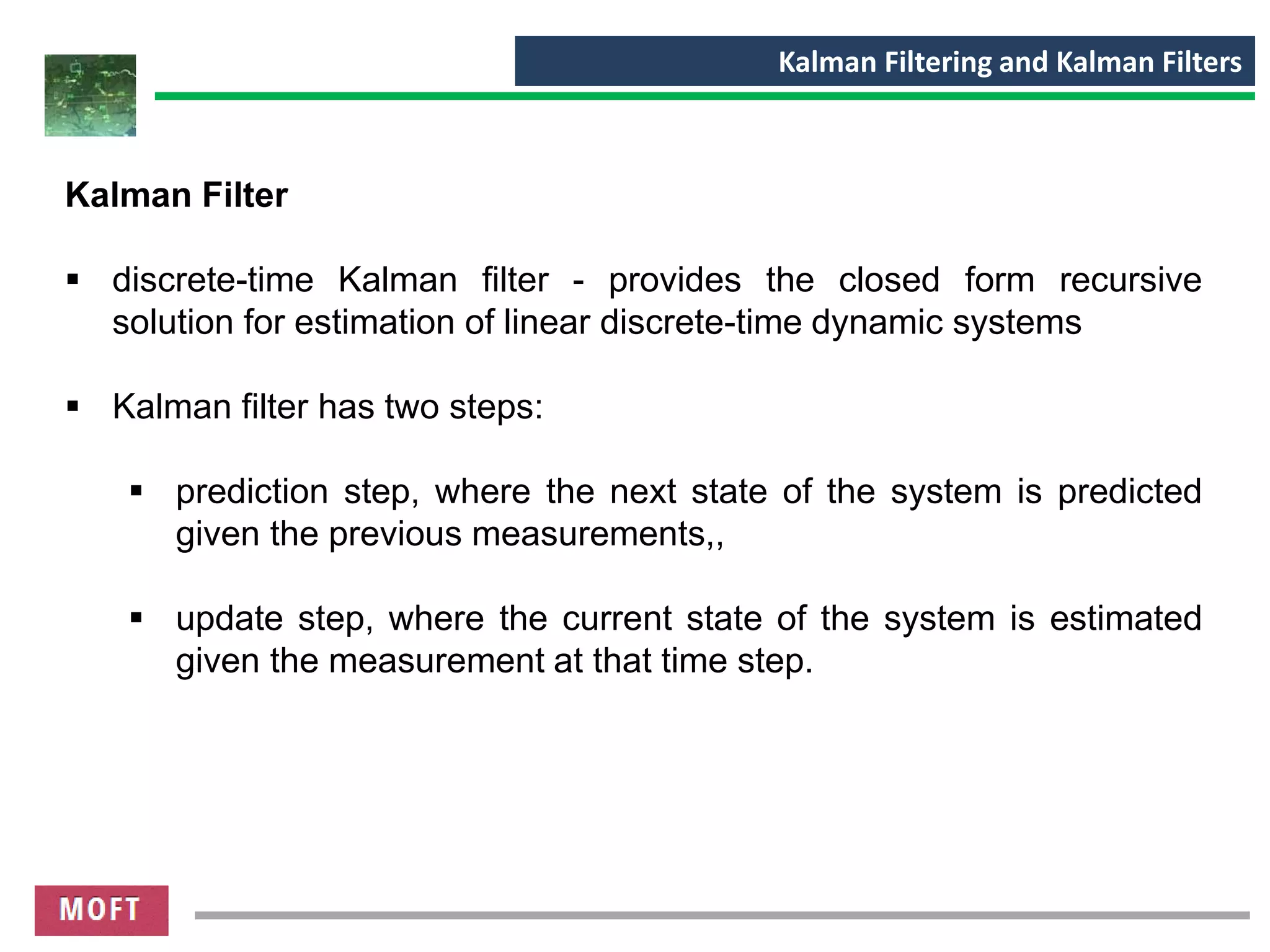
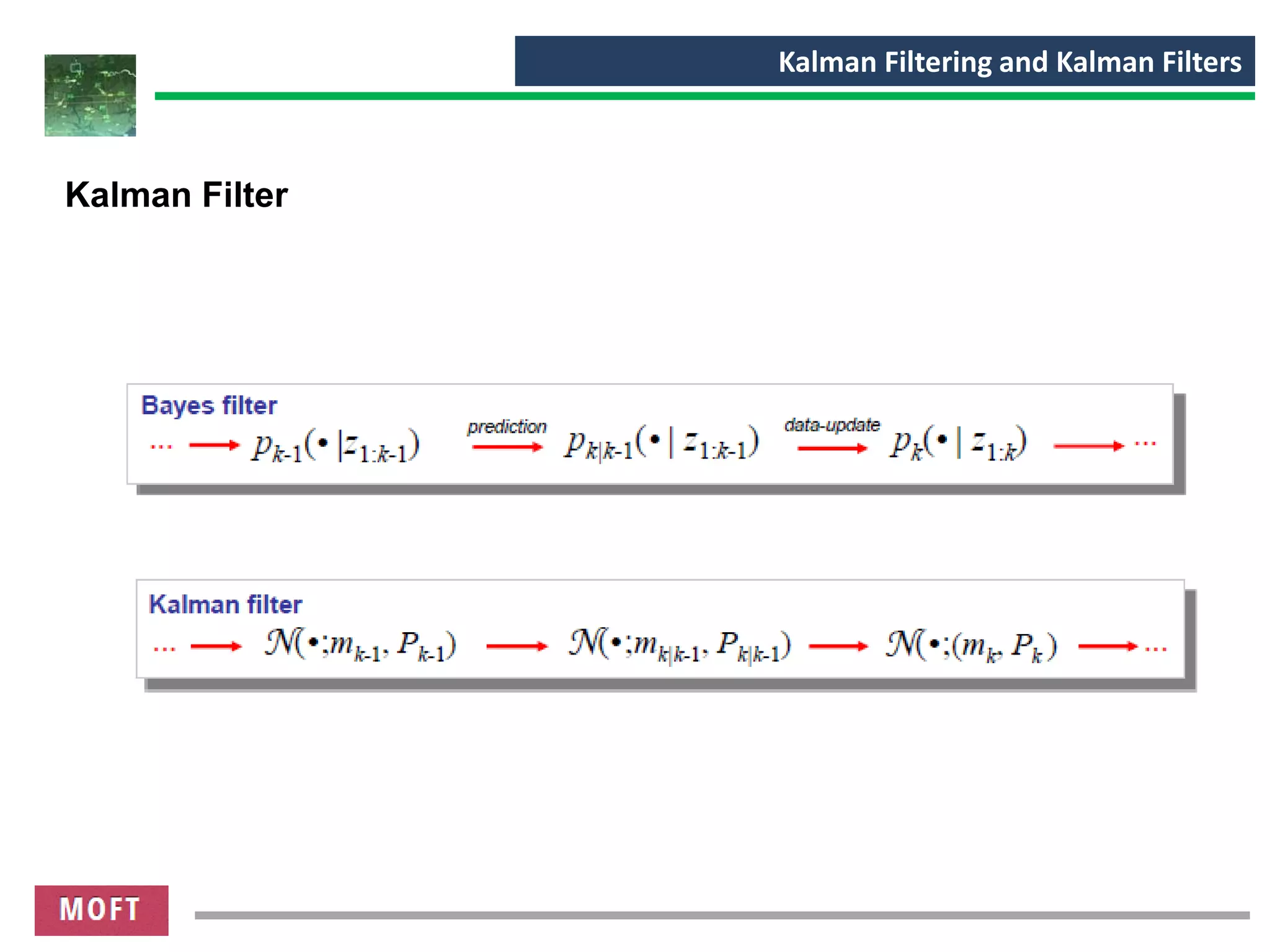
▪ discrete-time Kalman filter - provides the closed form recursive
solution for estimation of linear discrete-time dynamic systems
▪ Kalman filter has two steps:
▪ prediction step, where the next state of the system is predicted
given the previous measurements,,
▪ update step, where the current state of the system is estimated
given the measurement at that time step.
Kalman Filtering and Kalman Filters
Kalman Filter
Kalman Filtering and Kalman Filters
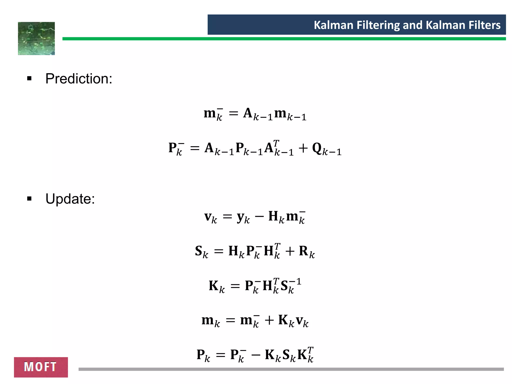
▪ Prediction:
𝐦 𝑘
−
= 𝐀 𝑘−1 𝐦 𝑘−1
𝐏𝑘
−
= 𝐀 𝑘−1 𝐏𝑘−1 𝐀 𝑘−1
𝑇
+ 𝐐 𝑘−1
▪ Update:
𝐯 𝑘 = 𝐲 𝑘 − 𝐇 𝑘 𝐦 𝑘
−
𝐒 𝑘 = 𝐇 𝑘 𝐏𝑘
−
𝐇 𝑘
𝑇
+ 𝐑 𝑘
𝐊 𝑘 = 𝐏𝑘
−
𝐇 𝑘
𝑇
𝐒 𝑘
−1
𝐦 𝑘 = 𝐦 𝑘
−
+ 𝐊 𝑘 𝐯 𝑘
𝐏𝑘 = 𝐏𝑘
−
− 𝐊 𝑘 𝐒 𝑘 𝐊 𝑘
𝑇
Kalman Filtering and Kalman Filters
• 𝐦 𝑘
−
and 𝐏𝑘
−
are the predicted mean and covariance of the state,
respectively, on the time step 𝑘 before seeing the measurement
• 𝐦 𝑘 and 𝐏𝑘 are the estimated mean and covariance of the state,
respectively, on time step 𝑘 after seeing the measurement
• 𝐯 𝑘 is the innovation or the measurement residual on time step 𝑘
• 𝐒 𝑘 is the measurement prediction covariance on the time step 𝑘
• 𝐊 𝑘 is the filter gain, which tells how much the predictions should be
corrected on time step 𝑘
Kalman Filtering and Kalman Filters
Kalman Filter
Kalman Filtering and Kalman Filters
▪ predicted and estimated state covariances on different time steps do
not depend on any measurements
▪ can be calculated off-line before making any measurements provided
that the matrices 𝐀, 𝐐, 𝐑 and 𝐇 are known on those particular time
steps
Kalman Filtering and Kalman Filters
Kalman Filter Variants
EKF - Extended Kalman Filter
▪ linearize model
▪ apply Kalman filtering equation to linearized model
Kalman Filtering and Kalman Filters
Kalman Filter Variants
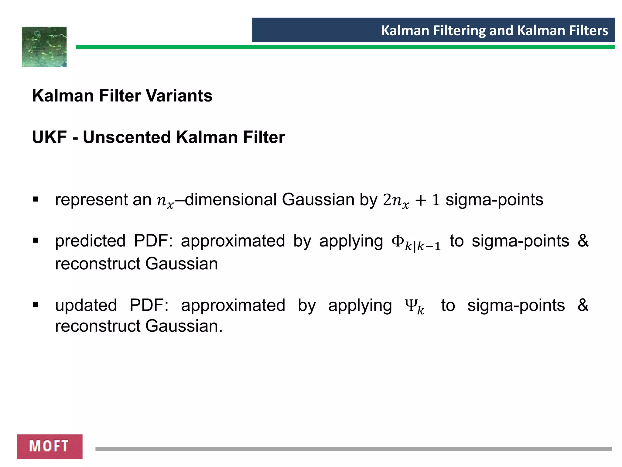
UKF - Unscented Kalman Filter
▪ represent an 𝑛 𝑥–dimensional Gaussian by 2𝑛 𝑥 + 1 sigma-points
▪ predicted PDF: approximated by applying Φ 𝑘|𝑘−1 to sigma-points &
reconstruct Gaussian
▪ updated PDF: approximated by applying Ψ𝑘 to sigma-points &
reconstruct Gaussian.
References
[1] Understanding and Applying Kalman Filtering, Lindsay Kleeman, Department
of Electrical and Computer Systems Engineering Monash University, Clayton
[2] Ba-Ngu Vo, Random Finite Set for Multi-object Dynamical System,
Department of ECE Curtin University Perth Western Australia
Other MOFT Tutorials – Lists and Links
Introduction to Multi Target Tracking
Bayesian Inference and Filtering
Kalman Filtering
Sequential Monte Carlo (SMC) Methods and Particle Filtering
Single Object Filtering Single Target Tracking
Nearest Neighbor(NN) and Probabilistic Data Association Filter(PDAF)
Multi Object Filtering Multi Target Tracking
Global Nearest Neighbor and Joint Probabilistic Data Association Filter
Data Association in Multi Target Tracking
Multiple Hypothesis Tracking, MHT
Other MOFT Tutorials – Lists and Links
Random Finite Sets, RFS
Random Finite Set Based RFS Filters
RFS Filters, Probability Hypothesis Density, PHD
RFS Filters, Cardinalized Probability Hypothesis Density, CPHD Filter
RFS Filters, Multi Bernoulli MemBer and Cardinality Balanced MeMBer, CBMemBer Filter
RFS Labeled Filters, Generalized Labeled Multi Bernoulli, GLMB and Labeled Multi Bernoulli, LMB Filters
Multiple Model Methods in Multi Target Tracking
Multi Target Tracking Implementation
Multi Target Tracking Performance and Metrics
http://www.egniya.com/EN/MOFT/Tutorials/
moft@egniya.com

Kalman Filtering

  • 1.
    MOFT Tutorials Multi ObjectFiltering Multi Target Tracking Kalman Filtering and Kalman Filters
  • 2.
    Kalman Filtering andKalman Filters Optimal Filtering ▪ methodology used for estimating the state of a time varying system, observed through noisy measurements ▪ state refers to the physical state ▪ described by dynamic variables, such as position, velocity and acceleration of a moving object ▪ noise in the measurements means a certain degree of uncertainty ▪ dynamic system evolves as a function of time, cannot be modelled entirely deterministically ▪ noise in the dynamics of system, process noise,
  • 3.
    Kalman Filtering andKalman Filters ▪ filtering means the process of filtering out the noise in the measurements ▪ and providing an optimal estimate for the state given the observed measurements and the assumptions made about the dynamic system
  • 4.
    Kalman Filtering andKalman Filters Discrete-Time State Space Models ▪ models where the states are defined on discrete time instances. ▪ defined recursively in terms of distributions 𝐱 𝑘~𝑝 𝐱 𝑘|𝐱 𝑘−1 𝐲 𝑘~𝑝 𝐲 𝑘|𝐱 𝑘
  • 5.
    Kalman Filtering andKalman Filters ▪ 𝐱 𝑘 ∈ ℝ 𝒏 is the state of the target on time step 𝑘, which can be, for example, the position, the velocity or the acceleration of the target. ▪ 𝐲 𝑘 ∈ ℝ 𝒎 is the measurement on time step 𝑘, which can be, for example, position of the target, distance to the target or the relative angle between the target and the sensor.
  • 6.
    Kalman Filtering andKalman Filters ▪ 𝑝 𝐱 𝑘|𝐱 𝑘−1 is the dynamic model which characterizes the dynamic behavior of the system ▪ usually the model is a probability density (continuous state), but it can also be a counting measure (discrete state), or a combination of them, if the state is both continuous and discrete. ▪ 𝑝 𝐲 𝑘|𝐱 𝑘 is the model for measurements, describes how the measurements are distributed given the state. ▪ model characterizes how the dynamic model is perceived by the observers
  • 7.
    Kalman Filtering andKalman Filters ▪ system defined this way has so called Markov-property, ▪ state 𝐱 𝑘 given 𝐱 𝑘−1 is independent from the history of states and measurements, ▪ expressed as; 𝑝 𝐱 𝑘|𝐱1:𝑘−1, 𝐲1:𝑘−1 = 𝑝 𝐱 𝑘|𝐱 𝑘−1 𝑝 𝐱 𝑘−1|𝐱 𝑘:𝑇, 𝐲 𝑘:𝑇 = 𝑝 𝐱 𝑘−1|𝐱 𝑘 ▪ measurement 𝐲 𝑘 is independent from the histories of measurements and states, ▪ expressed with equality 𝑝 𝐲 𝑘|𝐱1:𝑘, 𝐲1:𝑘−1 = 𝑝 𝐲 𝑘|𝐱 𝑘
  • 8.
    Kalman Filtering andKalman Filters General Dynamic Model and Measurement Model
  • 9.
    Kalman Filtering andKalman Filters General Dynamic Model and Measurement Model
  • 10.
    Kalman Filtering andKalman Filters ▪ problem - predicting and estimating dynamic system’s state given the measurements obtained so far ▪ predictive distribution for the state at the next time step 𝑝 𝐱 𝑘|𝐲1:𝑘−1 ▪ and marginal posterior distribution for the state at the current time step 𝑝 𝐱 𝑘|𝐲1:𝑘
  • 11.
    Kalman Filtering andKalman Filters Prediction-Update/ Predictor-Corrector Type Filtering
  • 12.
    Kalman Filtering andKalman Filters ▪ formal solutions for these distribution by recursive Bayesian filtering equations; 𝑝 𝐱 𝑘|𝐲1:𝑘−1 = න 𝑝 𝐱 𝑘|𝐱 𝑘−1 𝑝 𝐱 𝑘−1|𝐲1:𝑘−1 𝑑𝐱 𝑘−1 and 𝑝 𝐱 𝑘|𝐲 𝑘 = 1 𝑍 𝑘 𝑝 𝐲 𝑘|𝐱 𝑘 𝑝 𝐱 𝑘−1|𝐲1:𝑘−1 where the normalization constant 𝑍 𝑘 is given as 𝑍 𝑘 = න 𝑝 𝐲 𝑘|𝐱 𝑘 𝑝 𝐱 𝑘|𝐲1:𝑘−1 𝑑𝐱 𝑘
  • 13.
    Kalman Filtering andKalman Filters ▪ smoothed state estimates of previous time steps given the measurements obtained ▪ marginal posterior distribution 𝑝 𝐱 𝑘|𝐲1:𝑇 where 𝑇 > 𝑘. ▪ formal solution as a set of recursive Bayesian equations 𝑝 𝐱 𝑘+1|𝐲1:𝑘 = න 𝑝 𝐱 𝑘+1|𝐱 𝑘 𝑝 𝐱 𝑘|𝐲1:𝑘 𝑑𝐱 𝑘 𝑝 𝐱 𝑘|𝐲1:𝑇 = 𝑝 𝐱 𝑘|𝐲1:𝑘 න 𝑝 𝐱 𝑘+1|𝐱 𝑘 𝑝 𝐱 𝑘+1|𝐲1:𝑇 𝑝 𝐱 𝑘+1|𝐲1:𝑘 𝑑𝐱 𝑘+1
  • 14.
    Kalman Filtering andKalman Filters
  • 15.
    Kalman Filtering andKalman Filters Linear State Space Estimation ▪ simplest of the state space models - linear models of the following form: 𝐱 𝑘 = 𝐀 𝑘−1 𝐱 𝑘−1 + 𝐪 𝑘−1 𝐲 𝑘 = 𝐇 𝑘 𝐱 𝑘 + 𝐫𝑘 ▪ 𝐱 𝑘 ∈ ℝ 𝒏 is the state of the system on the time step 𝑘. ▪ 𝐲 𝑘 ∈ ℝ 𝒎 is the measurement on the time step 𝑘. ▪ 𝐪 𝑘−1 ~𝒩 𝟎, 𝐐 𝑘−1 is the process noise on the time step 𝑘 − 1. ▪ 𝐫𝑘 ~𝒩 𝟎, 𝐑 𝑘 is the measurement noise on the time step 𝑘. ▪ 𝐀 𝑘−1 is the transition matrix of the dynamic model. ▪ 𝐇 𝑘 is the measurement model matrix. ▪ prior distribution for the state is 𝐫𝑘 ~𝒩 𝐦0, 𝐏0 , where parameters 𝐦0 and 𝐏0 are set using the information known about the system
  • 16.
    Kalman Filtering andKalman Filters Linear State-Space Estimation
  • 17.
    Kalman Filtering andKalman Filters Linear State Space Estimation ▪ model equivalently expressed in probabilistic terms with distributions 𝑝 𝐱 𝑘|𝐱 𝑘−1 = 𝒩 𝐱 𝑘|𝐀 𝑘−1 𝐱 𝑘−1, 𝐐 𝑘−1 𝑝 𝐲 𝑘|𝐱 𝑘 = 𝒩 𝐱 𝑘|𝐇 𝑘 𝐱 𝑘−1, 𝐑 𝑘
  • 18.
    Kalman Filtering andKalman Filters Kalman Filter ▪ discrete-time Kalman filter - provides the closed form recursive solution for estimation of linear discrete-time dynamic systems ▪ Kalman filter has two steps: ▪ prediction step, where the next state of the system is predicted given the previous measurements,, ▪ update step, where the current state of the system is estimated given the measurement at that time step.
  • 19.
    Kalman Filtering andKalman Filters Kalman Filter
  • 20.
    Kalman Filtering andKalman Filters ▪ Prediction: 𝐦 𝑘 − = 𝐀 𝑘−1 𝐦 𝑘−1 𝐏𝑘 − = 𝐀 𝑘−1 𝐏𝑘−1 𝐀 𝑘−1 𝑇 + 𝐐 𝑘−1 ▪ Update: 𝐯 𝑘 = 𝐲 𝑘 − 𝐇 𝑘 𝐦 𝑘 − 𝐒 𝑘 = 𝐇 𝑘 𝐏𝑘 − 𝐇 𝑘 𝑇 + 𝐑 𝑘 𝐊 𝑘 = 𝐏𝑘 − 𝐇 𝑘 𝑇 𝐒 𝑘 −1 𝐦 𝑘 = 𝐦 𝑘 − + 𝐊 𝑘 𝐯 𝑘 𝐏𝑘 = 𝐏𝑘 − − 𝐊 𝑘 𝐒 𝑘 𝐊 𝑘 𝑇
  • 21.
    Kalman Filtering andKalman Filters • 𝐦 𝑘 − and 𝐏𝑘 − are the predicted mean and covariance of the state, respectively, on the time step 𝑘 before seeing the measurement • 𝐦 𝑘 and 𝐏𝑘 are the estimated mean and covariance of the state, respectively, on time step 𝑘 after seeing the measurement • 𝐯 𝑘 is the innovation or the measurement residual on time step 𝑘 • 𝐒 𝑘 is the measurement prediction covariance on the time step 𝑘 • 𝐊 𝑘 is the filter gain, which tells how much the predictions should be corrected on time step 𝑘
  • 22.
    Kalman Filtering andKalman Filters Kalman Filter
  • 23.
    Kalman Filtering andKalman Filters ▪ predicted and estimated state covariances on different time steps do not depend on any measurements ▪ can be calculated off-line before making any measurements provided that the matrices 𝐀, 𝐐, 𝐑 and 𝐇 are known on those particular time steps
  • 24.
    Kalman Filtering andKalman Filters Kalman Filter Variants EKF - Extended Kalman Filter ▪ linearize model ▪ apply Kalman filtering equation to linearized model
  • 25.
    Kalman Filtering andKalman Filters Kalman Filter Variants UKF - Unscented Kalman Filter ▪ represent an 𝑛 𝑥–dimensional Gaussian by 2𝑛 𝑥 + 1 sigma-points ▪ predicted PDF: approximated by applying Φ 𝑘|𝑘−1 to sigma-points & reconstruct Gaussian ▪ updated PDF: approximated by applying Ψ𝑘 to sigma-points & reconstruct Gaussian.
  • 26.
    References [1] Understanding andApplying Kalman Filtering, Lindsay Kleeman, Department of Electrical and Computer Systems Engineering Monash University, Clayton [2] Ba-Ngu Vo, Random Finite Set for Multi-object Dynamical System, Department of ECE Curtin University Perth Western Australia
  • 27.
    Other MOFT Tutorials– Lists and Links Introduction to Multi Target Tracking Bayesian Inference and Filtering Kalman Filtering Sequential Monte Carlo (SMC) Methods and Particle Filtering Single Object Filtering Single Target Tracking Nearest Neighbor(NN) and Probabilistic Data Association Filter(PDAF) Multi Object Filtering Multi Target Tracking Global Nearest Neighbor and Joint Probabilistic Data Association Filter Data Association in Multi Target Tracking Multiple Hypothesis Tracking, MHT
  • 28.
    Other MOFT Tutorials– Lists and Links Random Finite Sets, RFS Random Finite Set Based RFS Filters RFS Filters, Probability Hypothesis Density, PHD RFS Filters, Cardinalized Probability Hypothesis Density, CPHD Filter RFS Filters, Multi Bernoulli MemBer and Cardinality Balanced MeMBer, CBMemBer Filter RFS Labeled Filters, Generalized Labeled Multi Bernoulli, GLMB and Labeled Multi Bernoulli, LMB Filters Multiple Model Methods in Multi Target Tracking Multi Target Tracking Implementation Multi Target Tracking Performance and Metrics
  • 29.