This document discusses controllability and observability in the context of closed-loop control systems. It defines controllability as the ability to transfer a system from one state to another using input signals, and observability as the ability to determine the system state from output measurements. The document presents theorems for determining controllability and observability based on system matrices. It also discusses how state estimators can be used to estimate unobservable states and how controllers can be designed using pole placement to achieve stability and reference signal tracking.

1. Modelling and Control of Dynamic
Systems
Controllability and Observability
Sven Laur
University of Tartu

2. Closed-loop Controllers:
Basic Structure

3. Closed-loop control with state estimation
y[k]
u[k]
System
Controller
r[k]
Ĝ[z]
State
Estimator
The instability of a open loop controller is caused by gradual accumulation of
disturbances. The control signal becomes unsynchronised with the system.
⊲ If we can estimate the system state from the output, we can circumvent
such synchronisation errors. The system must be observable for that.
⊲ Even if we know the system state, it might be impossible to track the
reference signal. In brief, the system must be controllable.
1

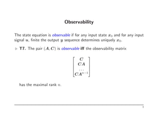
4. Controllability
The state equation is controllable if for any input state x0 and for any final
state x1 there exists an input u that transfers x0 to x1 in a finite time.
⊲ T6. The n dimensional pair (A, B) is controllable iff the controllability
matrix
B AB A2
B An−1
B
has the maximal rank n.
The desired input can be computed from the system of linear equations
x1 = An
x0 + An−1
Bu[0] + An−2
Bu[1] + · · · + Bu[n − 1] .
Although the theorem T6 gives an explicit method for controlling the
system, it is an off-line algorithm with a time lag n.
A good controller design should yield a faster and more robust method.
2

5. Observability
The state equation is observable if for any input state x0 and for any input
signal u, finite the output y sequence determines uniquely x0.
⊲ T7. The pair (A, C) is observable iff the observability matrix




C
CA
. . .
CAn−1




has the maximal rank n.
3

6. Offline state estimation algorithm
Again, the input state x0 can be computed from a system of linear equations













y[0] = Cx0 + Du[0]
y[1] = CAx0 + CBu[0] + Du[1]
· · ·
y[n − 1] = CAn−1
x0 + · · · + CBu[n − 2] + Du[n − 1]
Although this equation allows us to find out the state of the system, it is
offline algorithm, which provides a state estimation with a big time lag.
A good state space estimator must be fast and robust.
4

7. General structure of state estimators
y[k]
u[k] System
State Estimator
x̂[k]
x[k] = Ax[k − 1] + Bu[k − 1]
y[k] = Cx[k] + Du[k]
A state estimate x̂[k] is updated according to u[k] and y[k]:
⊲ Update rules are based on linear operations.
⊲ The state estimator must converge quickly to the true value x[k]
⊲ The state estimator must tolerate noise in the inputs u[k] and y[k].
5

8. Example
Consider a canonical realisation of the transfer function ĝ[z] = 0.5z+0.5
z2−0.25
A =
0 0.25
1 0
B =
1
0
C = [0.5 0.5] D = 0
Then a possible stable state estimator is following
x̂[k + 1] = Ax̂[k] + Bu[k] + 1(y[k] − Cx̂[k]
| {z }
ŷ[k]
) .
In general, the feedback vector 1 can be replaced with any other vector to
increase the stability of a state estimator.
6

9. Kalman Decomposition

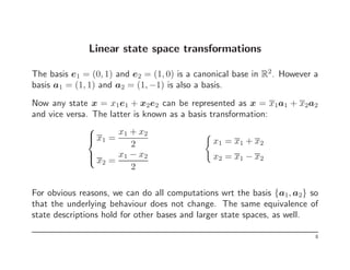
10. Equivalent state equations
Two different state descriptions of linear systems
(
x[k + 1] = A1x[k] + B1u[k]
y[k] = C1x[k] + D1u[k]
(
x[k + 1] = A2x[k] + B2u[k]
y[k] = C2x[k] + D2u[k]
are equivalent if for any initial state x0 there exists an initial state x0 such
that for any input u both systems yield the same output and vice versa.
⊲ T8. Two state descriptions are (algebraically) equivalent if there exists
an invertible matrix P such that
A2 = P A1P −1
B2 = P B1
C2 = C1P −1
D2 = D1 .
7

11. Linear state space transformations
The basis e1 = (0, 1) and e2 = (1, 0) is a canonical base in R2
. However a
basis a1 = (1, 1) and a2 = (1, −1) is also a basis.
Now any state x = x1e1 + x2e2 can be represented as x = x1a1 + x2a2
and vice versa. The latter is known as a basis transformation:





x1 =
x1 + x2
2
x2 =
x1 − x2
2
(
x1 = x1 + x2
x2 = x1 − x2
For obvious reasons, we can do all computations wrt the basis {a1, a2} so
that the underlying behaviour does not change. The same equivalence of
state descriptions hold for other bases and larger state spaces, as well.
8

12. Kalman decomposition
⊲ T9. Every state space equation can be transformed into an equivalent
description to a canonical form




xco[k + 1]
xco[k + 1]
xco[k + 1]
xco[k + 1]



 =




Aco 0 A13 0
A21 Aco A23 A24
0 0 Aco 0
0 0 A43 Aco








xco[k]
xco[k]
xco[k]
xco[k]



 +




Bco
Bco
0
0



 u[k]
y[k] = [Cco 0 Cco 0] x[k] + Du[k]
where
⋄ xco is controllable and observable
⋄ xco is controllable but not observable
⋄ xco is observable but not controllable
⋄ xco is neither controllable nor observable
9

13. Minimal realisation
⊲ T10. All minimal realisations are controllable and observable. A
realisation of a proper transfer function ĝ[z] = N(z)/D(z) is minimal iff
it state space dimension dim(x0) = deg D(z).
10

14. Closed-loop Controllers:
Design Principles

15. General setting
According to Kalman decomposition theorem, the state variables can be
divided into four classes depending on controllability and observability.
⊲ We cannot do anything with non-controllable state variables.
⊲ Non-observable variables can be controlled only if they are marginally
stable. We can do it with an open-loop controller.
⊲ For controllable and observable state variables, we can build effective
closed-loop controllers.
Simplifying assumptions
⊲ From now on, we assume that we always want to control state variables
that are both controllable and directly observable: y[k] = x[k].
⊲ If this is not the case, then we must use state estimators to get an
estimate of x. The latter just complicates the analysis.
11

16. Unity-feedback configuration
y[k]
u[k] System
Controller
r[k]
ĝ[z]
Ĉ[z]
p +
-1
Design tasks
⊲ Find a compensator ĉ[z] such that system becomes stable.
⊲ Find a proper value of p such that system starts to track reference signal.
It is sometimes impossible to find p such that y[k] ≈ r[k].
⊲ The latter is impossible if ĝ[1] = 0, then the output y[k] just dies out.
12

17. Overall transfer function
Now note that
ŷ = ĝ[z]ĉ[z](pr̂ − ŷ) ⇐⇒ ŷ =
pĝ[z]ĉ[z]
1 + ĝ[z]ĉ[z]
r̂
and thus the configuration is stable when the new transfer function
ĝ◦[z] =
pĝ[z]ĉ[z]
1 + ĝ[z]ĉ[z]
has poles lying in the unit circle. Now observe
ĝ[z] =
N(z)
D(z)
, ĉ[z] =
B(z)
A(z)
=⇒ ĝ◦[z] =
pB(z)N(z)
A(z)D(z) + B(z)N(z)
13

18. Pole placement
We can control the denominator of the new transfer function ĝ◦[z]. Let
F(z) = A(z)D(z) + B(z)N(z)
be a desired new denominator. Then there exists polynomials A(z) and
B(z) for every polynomial F(z) provided that D(z) and N(z) are coprime.
The degrees of the polynomials satisfy deg B(z) ≥ deg F(z) − deg D(z).
ℑ(s)
ℜ(s)
BIBO
stable
ℜ(z)
ℑ(z)
BIBO
stable
14

19. Signal tracking properties
Let ĝ◦[z] be the overall transfer function.
⊲ The system stabilises if ĝ◦[z] is BIBO stable.
⊲ The system can track a constant signal r[k] ≡ a if ĝ◦[1] = 1.
⊲ The system can track a ramp signal r[k] ≡ ak if ĝ◦[1] = 1 and ĝ′
◦[1] = 0.
The latter follows from the asymptotic convergence
y[k] → aĝ′
◦[1] + kaĝ◦[1]
for an input signal r[k] = ak. Moreover, let ĝ◦ = N(z)/D(z). Then
ĝ◦[1] = 1 ∧ ĝ′
◦[1] = 0 ⇐⇒ N(1) = D(1) ∧ N′
(1) = D′
(1) .
15

20. Trade-offs in pole placement
A pole placement is a trade-off between three design criteria:
⊲ response time
⊲ overshoot ratio
⊲ maximal strength of the input signal
There is no general recipe for pole placement. Rules of thumb are given in
⊲ C.-T. Chen. Linear System Theory and Design. page 238.
16

21. Illustrative example
Consider a feedback loop with the transfer function g[z] = 1
z−2. Then we
can try many different pole placements
F(z) ∈
z − 0.5, z + 0.5, z2
− 0.25, z2
+ z + 0.25, z2
− z + 0.25
The corresponding compensators are
ĉ[z] ∈
3
2
,
5
2
,
15
4z + 8
,
24
4z + 12
,
9
4z + 4
,
p ∈
1
3
,
3
5
,
1
5
, ,
9
25
,
1
9
.
They can be found systematically by solving a system of linear equations.
17

22. Robust signal tracking
Sometimes the system changes during the operation. The latter can be
modelled as an additional additive term w[k] in the input signal.
If we know the poles of reference signal r[k] and w[k] ahead, then we can
design a compensator that filters out the error signal w[k].
For instance, if w[k] is a constant bias, then adding an extra pole 1
z−1
cancels out the effect of bias. See pages 277–283 for further examples.
In our example, the robust compensator for F[z] = z2
− 0.25 is
ĉ[z] =
12z − 9
4z − 4
p = 1 .
18

23. Model matching
Find a feedback configuration such that ĝ◦ is BIBO stable and ĝ◦[1] = 1.
y[k]
u[k] System
r[k]
ĝ[z]
Controller
ĉ1[z]
+
ĉ2[z]
Feedback
⊲ The two-parameter configuration described above provides more flexibility
and it is possible to cancel out zeroes that prohibit tracking.
⊲ There are many alternative configurations. A controller design is
acceptable if every closed-loop configuration is BIBO stable.
19