

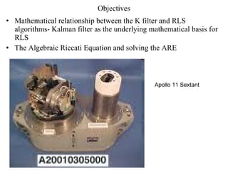


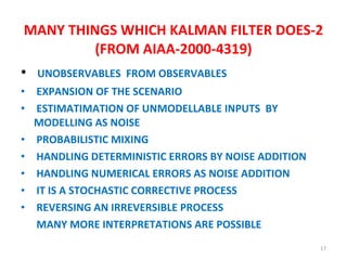


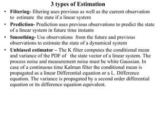
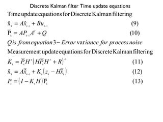
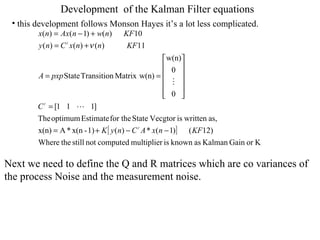
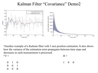
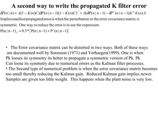
![Setting up the plant >> A = [ 1.1269 -0.4940 0.1129; 1 0 0 ; 0 1 0 ]; >> A A = 1.1269 -0.4940 0.1129 1.0000 0 0 0 1.0000 0 >> B = [ -0.3832; 0.5919; 0.5191]; >> C = [ 1 0 0]; >> Bp = B'; >> Bp Bp = -0.3832 0.5919 0.5191 >> Plant = ss(A,[B B],C,0,-1,'inputname',{'u' 'w'}, 'outputname‘’,'y1‘,’y2’}); Q = 1; R = 1; [kalmf,L,P,K] = kalman(Plant,Q,R); >> K K = 0.3798 0.0817 -0.2570 K is really the Kalman gain](https://image.slidesharecdn.com/kalmanequations-12831032637335-phpapp01/85/Kalman-Equations-25-320.jpg)
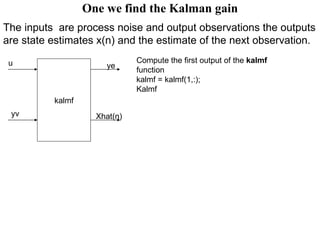

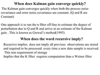


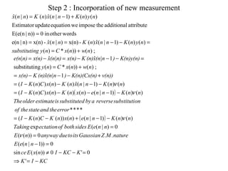


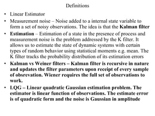
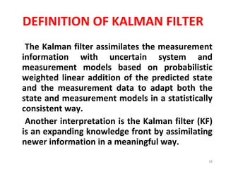
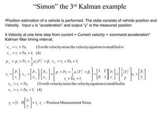
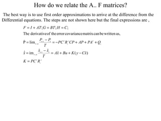
![This example directly applies K equations %Calculate the rest of the values. for j=2:nlen, %Calculate the state and the output x(j)=a*x(j-1)+w(j); z(j)=h*x(j)+v(j); %Predictor equations xapriori(j)=a*xaposteriori(j-1); residual(j)=z(j)-h*xapriori(j); papriori(j)=a*a*paposteriori(j-1)+Q; %Corrector equations k(j)=h*papriori(j)/(h*h*papriori(j)+R); paposteriori(j)=papriori(j)*(1-h*k(j)); xaposteriori(j)=xapriori(j)+k(j)*residual(j); end j=1:nlen; subplot(221); %Plot states and state estimates h1=stem(j+0.25,xapriori,'b'); hold on h2=stem(j+0.5,xaposteriori,'g'); h3=stem(j,x,'r'); hold off %Make nice formatting. legend([h1(1) h2(1) h3(1)],'a priori','a posteriori','exact'); title('State with a priori and a posteriori elements'); ylabel('State, x'); xlim=[0 length(j)+1]; set(gca,'XLim',xlim); subplot(223); %Plot errors h1=stem(j,x-xapriori,'b'); hold on h2=stem(j,x-xaposteriori,'g'); hold off legend([h1(1) h2(1)],'a priori','a posteriori'); title('Actual a priori and a posteriori error'); ylabel('Errors'); set(gca,'XLim',xlim); %Set limits the same as first graph](https://image.slidesharecdn.com/kalmanequations-12831032637335-phpapp01/85/Kalman-Equations-49-320.jpg)
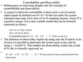
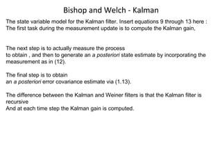
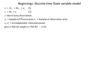
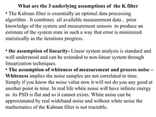
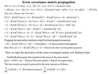
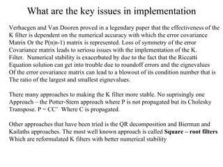
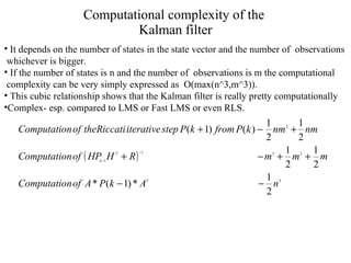
![This example directly applies K equations %Plot errors subplot(223); h1=stem(j,x-xapriori,'b'); hold on h2=stem(j,x-xaposteriori,'g'); hold off legend([h1(1) h2(1)],'a priori','a posteriori'); title('Actual a priori and a posteriori error'); ylabel('Errors'); set(gca,'XLim',xlim); %Set limits the same as first graph %Plot kalman gain, k subplot(224); h1=stem(j,k,'b'); legend([h1(1)],'kalman gain'); title('Kalman gain'); ylabel('Kalman gain, k'); set(gca,'XLim',xlim); %Set limits the same as first graph](https://image.slidesharecdn.com/kalmanequations-12831032637335-phpapp01/85/Kalman-Equations-50-320.jpg)

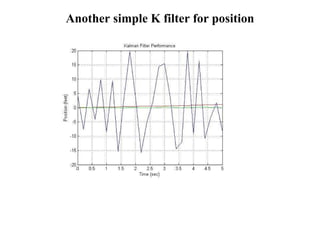
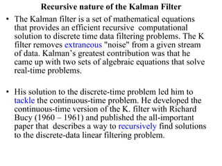
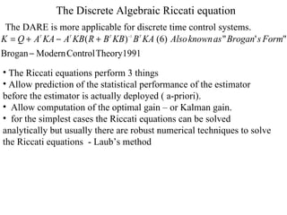
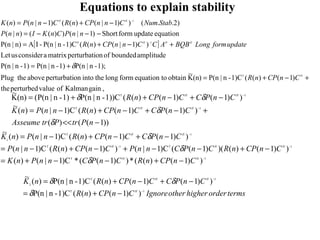
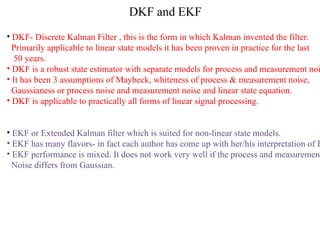
![Kalman demo 1 duration=5; dt=0.2; [pos,posmeas,poshat]= kalman_demo1(duration,dt); Kalman_demo1 function is available from the instructor](https://image.slidesharecdn.com/kalmanequations-12831032637335-phpapp01/85/Kalman-Equations-53-320.jpg)
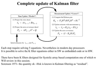
![A 4x4 Kalman filter example This example includes a 4x4 estimator for a movement of a point in 2 –dimensional Plane starting from (10,10) . Consider a particle moving in the plane at constant velocity subject to random perturbations in its trajectory. The new position (x1, x2) is the old position plus the velocity (dx1, dx2) plus noise w. [ x1(t) ] = [1 0 1 0] [ x1(t-1) ] + [ wx1 ] [ x2(t) ] [0 1 0 1] [ x2(t-1) ] +[ wx2 ] [ dx1(t) ] [0 0 1 0] [ dx1(t-1) ] +[ wdx1 ] [ dx2(t) ] [0 0 0 1] [ dx2(t-1) ]+ [ wdx2 ] We assume we only observe the position of the particle. [ y1(t) ] = [1 0 0 0] [ x1(t) ] + [ vx1 ] [ y2(t) ] [0 1 0 0] [ x2(t) ]+ [ vx2 ] [ dx1(t) ] [ dx2(t) ] Plant = ss(A,[B B],C,0,-1,'inputname',{'u' 'w'}, 'outputname‘’,'y1‘,’y2’}); [x,y] = sample_lds(F, H, Q, R, initx, T); [xfilt, Vfilt, VVfilt, loglik] = kalman_filter(y, F, H, Q, R, initx, initV);](https://image.slidesharecdn.com/kalmanequations-12831032637335-phpapp01/85/Kalman-Equations-54-320.jpg)
![>> F = [1 0 1 0; 0 1 0 1; 0 0 1 0; 0 0 0 1]; H = [1 0 0 0; 0 1 0 0]; Q = 0.1*eye(ss); R = 1*eye(os); >> F F =1 0 1 0 0 1 0 1 0 0 1 0 0 0 0 1](https://image.slidesharecdn.com/kalmanequations-12831032637335-phpapp01/85/Kalman-Equations-55-320.jpg)
![Building the F, H, G matrices T =.0.1sec; F= H = [ 1 0]; A = [ 1 0.1; 0 1]; B = [ 0.005; 0.1]; C = [ 1 0]; Xinit = [0;0];x = Xinit; xhat= Xinit; % Initital state estimate R = measnoise^2; % R matrix Sw = accelnoise^2*[ 1 0 ; 0 1]; % Q matrix P = Sw; % Defintion Position vector and Poistion estimated vectors pos = []; poshat = []; posmeas= []; vel = []; velhat = []; duration = 10;](https://image.slidesharecdn.com/kalmanequations-12831032637335-phpapp01/85/Kalman-Equations-58-320.jpg)
![Kalman Position Tracker for t = 0:dt:duration u = 1; % Simulate the Linear system Processnoise = accelnoise*[(dt^2/2)*randn; dt*randn]; x = A*x + B*u + Processnoise; % Simulate the obserbvation equation y = C*x + measnoise; % Update the state Estimate xhat = A*xhat +B*u; % Form the Innovation Vector Inno_vec = y - C*xhat; % Write the equation for Compuation of th Covariance of Innovations % Process S = C*P*C' + Sz; % Use the computed Covariance of Innovation to comnpute the Kalaman Gain% Gain K = A*P*C'*inv(S); % Update the State Estimate xhat = xhat + K*Inno_vec; % Compute the covariance of the EStimation Error P = A*P*A' -A*P*C'*inv(S)*C*P*A' + Sw; pos = [pos; x(1)]; posmeas = [posmeas; y]; poshat = [poshat; xhat(1)]; vel = [vel; x(2)]; velhat = [velhat; xhat(2)]; End close all; t = [0:dt:duration]; figure(1); Sw = 0.5*accelnoise^2*[ 1 0 ; 0 1]; % Q matrix P = Sw; plot(t,pos','b', t,posmeas','g',t,poshat','r');](https://image.slidesharecdn.com/kalmanequations-12831032637335-phpapp01/85/Kalman-Equations-59-320.jpg)


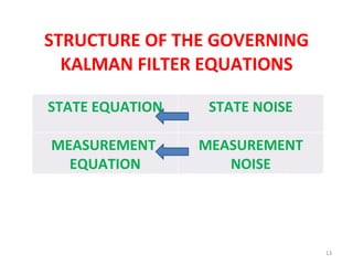
The document discusses Rudolf Kalman and his development of the Kalman filter, a mathematical method widely used in fields such as electrical engineering, mechanical engineering, and communications. It provides background on Kalman, an overview of the Kalman filter and how it works, and examples of its applications, notably in enabling the Apollo 11 moon landing through its use in the spacecraft's guidance system. The Kalman filter provides an efficient recursive solution to problems of discrete-time data filtering and estimation in dynamic systems with random noise.