Download as PDF, PPTX

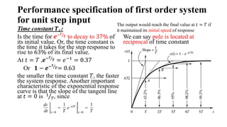
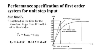
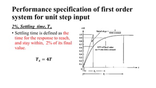
![Performance specification of first order
system for unit step input
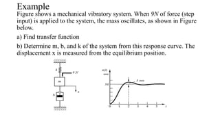
Example [page 160, Norman Nise]
A system has a transfer function, 𝐺 𝑠 =
50
𝑠+50
. Find the time constant,
𝑇𝑐 settling time,𝑇𝑠 and rise time,𝑇𝑟 of it’s step response.
Ans:
𝑇𝑐 = 0.02 s
𝑇𝑠 = 0.08 𝑠
𝑇𝑟 = 0.044 𝑠](https://image.slidesharecdn.com/ch3response-240426071756-40b72bdd/85/Transient-and-Steady-State-Response-Control-Systems-Engineering-17-320.jpg)
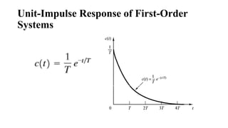
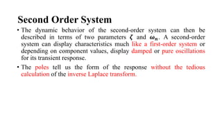
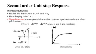
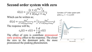
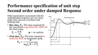
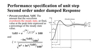
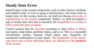
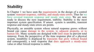


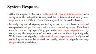
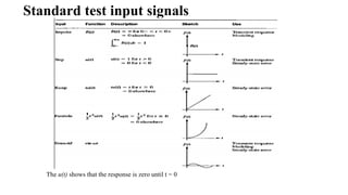
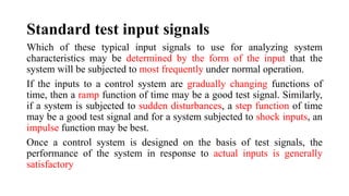
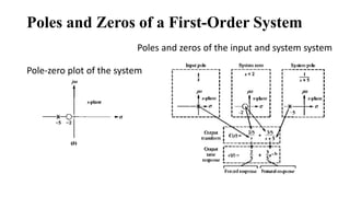
The document discusses the analysis of transient and steady-state responses in control systems, emphasizing the importance of test input signals such as impulse, step, ramp, parabolic, and sinusoidal for evaluating system performance. It explains how to determine system response characteristics, including poles and zeros, and describes the behavior of first- and second-order systems, including performance metrics like rise time, settling time, and steady-state error. Additionally, it categorizes control systems based on their ability to follow different input types and discusses the impact of system imperfections on steady-state errors.