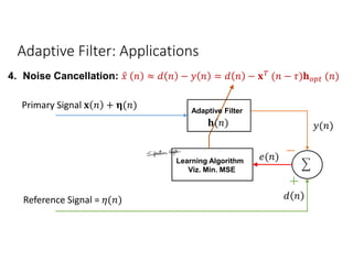
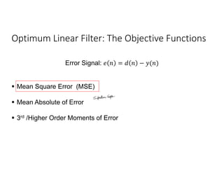
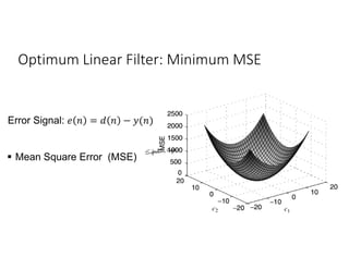
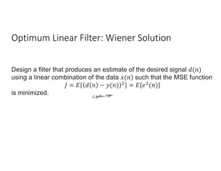
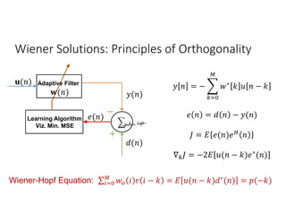
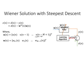
Adaptive filters are time-variant, nonlinear, and stochastic systems that perform data-driven approximation to minimize an objective function. The chapter discusses adaptive filter applications like system identification, inverse modeling, linear prediction, and noise cancellation. It also covers stochastic signal models, optimum linear filtering techniques like Wiener filtering, and solutions to the Wiener-Hopf equations. Numerical techniques like steepest descent are discussed for minimizing the mean square error function in adaptive filters. Stability and convergence analysis is presented for the steepest descent approach.

1. Chapter-4: Adaptive Signal Processing

2. Adaptive Signal Processing: Adaptive Filter
General Concept
 Adaptive Filters (AF) are, by design,
time-variant, nonlinear, and stochastic
systems
 The adaptive filter performs a data-
driven approximation step
 The environment to AF comprises of
• The input signal(s)
• The reference signal(s)
In cases where any of them is not well
defined, the design procedure is to
model the signals and subsequently
design the filter

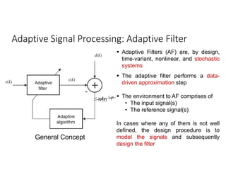
3. Adaptive Signal Processing: Adaptive Algorithm
General Concept
 The basic objective of the
adaptive/learning Algorithm is
• To set adaptive filter coefficients
(parameters) to minimize a
meaningful objective function
involving the input, the reference
signal, and adaptive filter output
signals
 The meaningful objective function
should be –
• Non-negative:
, , ≥ 0,
∀ ( ), ( ), ( ) ;
• Optimal: [ ( ), ( ), ( )] = 0.

4. Adaptive Filter: Applications
1. System Identification: ( ) ≈ ( )
Plant / System
Adaptive Filter
Learning Algorithm
Viz. Min. MSE
( )
( )
( )
( )
( )
( )

5. Adaptive Filter: Applications
2. Inverse Model: ( ) ≈ ( )
( )
Learning Algorithm
Viz. Min. MSE
( )
( )
( )
Adaptive Filter
( )
Plant / System
( )
Delay
( )

6. Adaptive Filter: Applications
3. Linear Prediction: ≈ = ( − ) ( )
( )
Learning Algorithm
Viz. Min. MSE
( )
= ( )
( )
Adaptive Filter
( )
Delay
( − )

7. Adaptive Filter: Applications
4. Noise Cancellation: ≈ − = − ( − ) ( )
Primary Signal + ( )
Learning Algorithm
Viz. Min. MSE
( )
( )
Adaptive Filter
( )
Reference Signal = ( )

8. Stochastic/Random Signal Models
• Driving question:
Can we generate random process of desired statistical
characteristics from statistically independent random process or
vice versa?

9. Stochastic Models
• General or Auto-regressive Moving Average (ARMA) Model
, [ ]
[ ] [ ]
= [ − ] − [ − ]

10. Stochastic Models
• Moving Average (MA) Model
ℎ
[ ] [ ]
= ℎ [ − ]

11. Stochastic Models
• Auto-regressive (AR) Model
ℎ[ ]
[ ] [ ]
= − ℎ − + [ ]

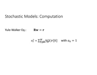
12. Stochastic Models: Computation
• Given the desired auto-correlation sequence for = 0, 1, 2, … ,
determine the ℎ( ) and the input process variance
ℎ − = [ ]
Yule-Walker Eq.: ∑ ℎ∗
− = 0 for > 0
∑ ℎ∗
− = for = 0

13. Stochastic Models: Computation
Yule-Walker Eq.: =
= ∑ ℎ( ) with = 1

14. Optimum Linear Filter: Filter Structures
 Finite Impulse Response
• Direct Form-I
• Direct Form-II
• Lattice Structure
 Infinite Impulse Response
• Direct Form-I
• Direct Form-II
• Lattice Structure

15. Optimum Linear Filter: The Objective Functions
Error Signal: = − ( )
 Mean Square Error (MSE)
 Mean Absolute of Error
 3rd /Higher Order Moments of Error

16. Optimum Linear Filter: Minimum MSE
Error Signal: = − ( )
 Mean Square Error (MSE)

17. Optimum Linear Filter: Wiener Solution
Design a filter that produces an estimate of the desired signal ( )
using a linear combination of the data ( ) such that the MSE function
= − ( ) = ( )
is minimized.

18. Wiener Solutions
1. Principles of Orthogonality
2. MSE Surface Analysis
Both are leading to Wiener-
Hopf Equation

19. Wiener Solutions: Principles of Orthogonality
Learning Algorithm
Viz. Min. MSE
( )
( )
( )
Adaptive Filter
( )
( )
= − ∗
−
= − ( )
= ( )
∇ = −2 ( − ) ∗
( )
Wiener-Hopf Equation: ∑ − = ( − ) ∗
( ) = (− )

20. Wiener Solutions: Principles of Orthogonality
Wiener-Hopf Equation:
∑ − = ( − ) ∗
( ) = (− )
=
Where,
= ( ) ( )
= ( ) ∗
( )
=

21. Wiener Solutions: MSE Surface Analysis
= − − +
Minimizing w.r.t
=
Where,
= ( ) ( )
= ( ) ∗
( )
=

22. Wiener Solutions: Minimum MSE
= −
= −
( )
( )
( )
= 1 −
∈ = 1 −
0 ≤∈≤ 1

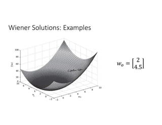
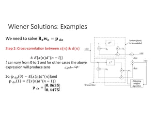
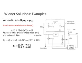
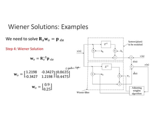
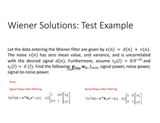
23. Wiener Solutions: Examples
Consider the sample autocorrelation coefficients ( (0) = 1.0, (1) = 0) from given
data ( ), which, in addition to noise, contain the desired signal. Furthermore,
assume the variance of the desired signal = 24.40 and the cross-correlation
vector be = [2 4.5] . It is desired to find the surface defined by the mean-
square function ( ).

24. Wiener Solutions: Examples
=
2
4.5

25. Wiener Solutions: Examples
Let us consider a plant model = 0.9 and
= 0.25 as shown in the figure. The plant
output are corrupted by a white noise
{ ( )} of zero mean and variance 2
= 0.15.
Find the Wiener coefficients and that
approximate (models) with following two
WSS processes as input which are
uncorrelated with ( ).
a. ( ) with zero mean and variance =
1.
b. ( ) with mean = 0.5 and variance =
0.64.

26. Wiener Solutions: Examples
We need to solve =
Step 1: What is ( ) in terms of ( )
Step 2: Cross-correlation between ( ) &
( )
Step 3: Auto-correlation matrix ( )
Step 4: Wiener Solution

27. Wiener Solutions: Examples
We need to solve =
Step 1: What is ( ) in terms of ( )
Given = 0.9 and = 0.25.
= 0.9 + 0.25 − 1 + ( )
Step 2: Cross-correlation between ( ) &
( )
≜ ( ) ∗( − )
can vary from 0 to 1 and for other cases
the above expression will produce zero

28. Wiener Solutions: Examples
We need to solve =
Step 2: Cross-correlation between ( ) & ( )
≜ ( ) ∗
( − )
can vary from 0 to 1 and for other cases the above
expression will produce zero
So, 0 = ( ) ∗
( ) and
1 = ( ) ∗
( − 1)
=
.
.

29. Wiener Solutions: Examples
We need to solve =
Step 3: Auto-correlation matrix ( )
( ) ≜ ( ) ∗
( − )
As ( ) is white process whose mean is 0.5
and variance is 0.64.
So, = + 0.5 = + 0.25
=
. .
. .

30. Wiener Solutions: Examples
We need to solve =
Step 4: Wiener Solution
=
=
1.2198 -0.3427
-0.3427 1.2198
0.8635
0.4475
=
0.9
0.25

31. Wiener Solutions: Generating Color Process
₊ ₊
+ ₊
( )
( )
x( )
+ +
A WSS process x is to
generated from a white process
( ) as shown in the figure.
The white process ( ) has
variance = 0.12. The auto-
correlation sequence of x is
0 = 1.0645 , 1 =
0.4925, 2 = 0.7665.
Determine , , and

32. Wiener Solutions: Generating Color Process
₊ ₊
+ ₊
( )
( )
x( )
+ +
Step 1: Determine s( ) in terms
of ( ) and expression of
autocorrelation sequence
Step 2: Determine auto-
correlation sequence of s( )
from that given for x( )
Step 3: Develop the Yule-
Walker equation
Step 4: Develop input variance
equation and solve for all
s( )
u( )

33. Wiener Solutions: Generating Color Process
₊ ₊
+ ₊
( )
( )
x( )
+ +
Step 1: Determine s( ) in terms
of ( )
− + − 1 …
+ − 2 = ( )
So,
− + − 1 …
+ − 2 =
∗
− = ( )
s( )
u( )

34. Wiener Solutions: Generating Color Process
₊ ₊
+ ₊
( )
( )
x( )
+ +
Step 2: Determine auto-
correlation sequence of s( )
from that given for x( )
= −
= − ( )
s( )
u( )

35. Wiener Solutions: Generating Color Process
₊ ₊
+ ₊
( )
( )
x( )
+ +
Step 3: Develop the Yule-Walker
equation
(0) (−1)
(1) (0)
−
=
− (1)
− (2)
= + and =
s( )
u( )

36. Wiener Solutions: Generating Color Process
₊ ₊
+ ₊
( )
( )
x( )
+ +
Step 4: Develop input variance
equation and solve for all
= 0 − 1 + 2
s( )
u( )

37. Wiener Solutions: Test Example
Let the data entering the Wiener filter are given by ( ) = ( ) + ( ).
The noise ( ) has zero mean value, unit variance, and is uncorrelated
with the desired signal ( ). Furthermore, assume ( ) = 0.9 and
( ) = ( ). Find the following: , , , signal power, noise power,
signal-to-noise power.
Hints:
Signal Power after filtering Noise Power after filtering

38. Wiener Solution with Steepest Descent
Numerical approach needs a recursive expression to minimize ( )
+ 1 = − ( )
Where, = ∇ =
( )
, is step size
Applying Taylor series expansion around + 1 up to 1st order
+ 1 ≈ + ( ) ( )
≈ − ( )
So, if is +ve, + 1 < for all

39. Wiener Solution with Steepest Descent
Learning
Algorithm
( )
( )
( )
Adaptive
Filter
( )
( )
= − ( )
= − ( )
Where,
= ( ) ( − 1) … ( − + 1)
= ( ) ( ) … ( )

40. Wiener Solution with Steepest Descent
Learning
Algorithm
( )
( )
( )
Adaptive
Filter
( )
( )
= − − +
=
( )
( )
⋮
( )
= −2 + 2 ( )
+ 1 = − − + ( )

41. Wiener Solution with Steepest Descent
+ 1 = + − ( )
( ) ( + 1)
 Stability Analysis
 What is the condition
that + 1 will
converge to ?
 Transient Behavior
 What is the rate of
convergence?

42. Minimum MSE Surface
= − − +
= −
So,
− = − − +
= + − −

43. Stability Analysis
Let deviation from optimal solution
n + 1 = − (n + 1)
n + 1 = − (n)
We can transform into Eigen space of as n = (n),
n + 1 = − Λ (n)
Then,
n + 1 = 1 − (0)
n + 1 → 0 as → ∞ if −1 < 1 − < 1
i.e. 0 < <

44. Transient Behavior
n + 1 = 1 − (0)
Time constant can be defined such that
1 − =
i.e. =
( )
≈ for ≪ 1