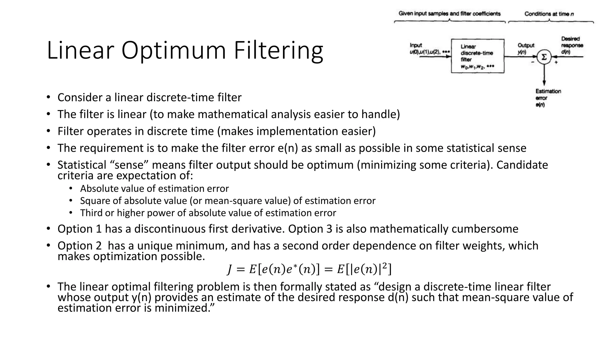
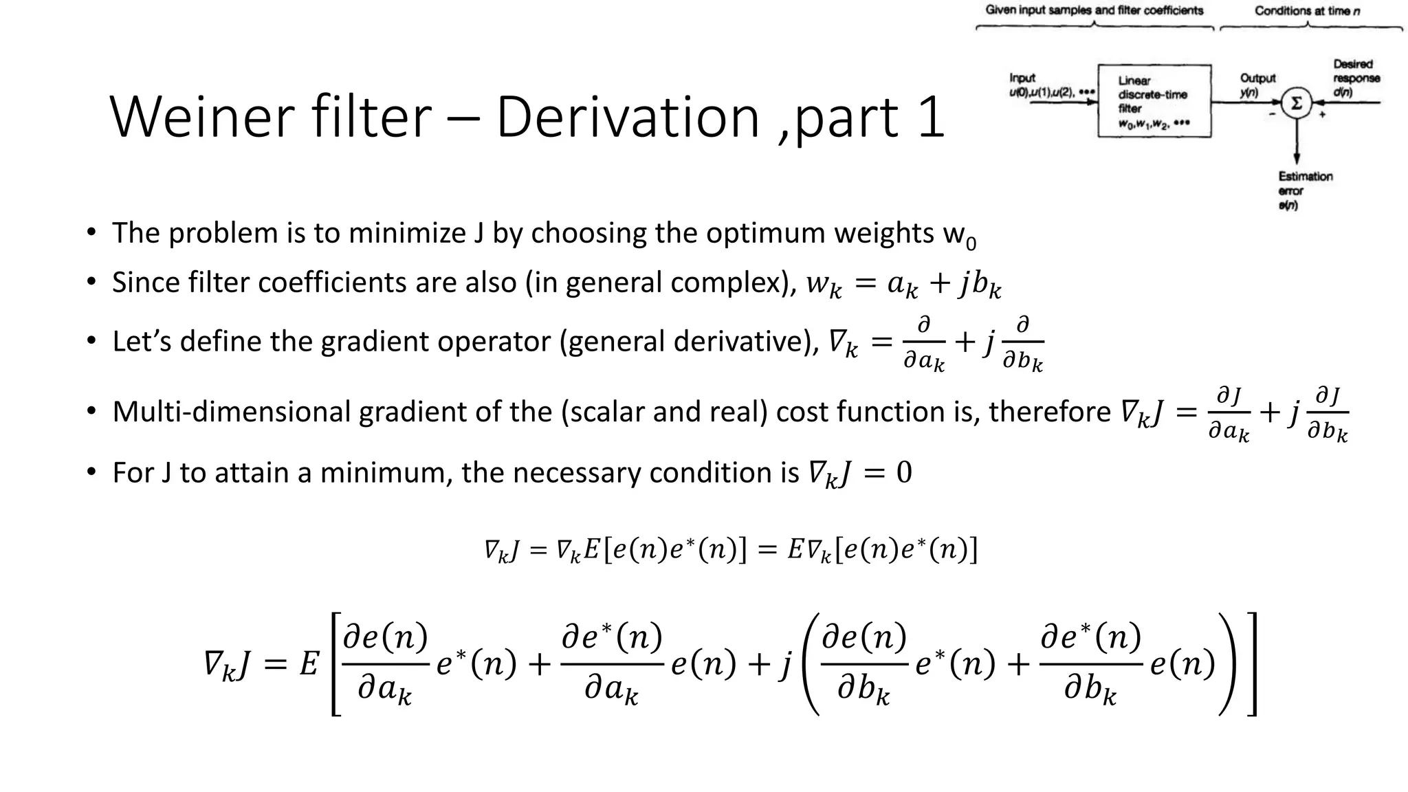
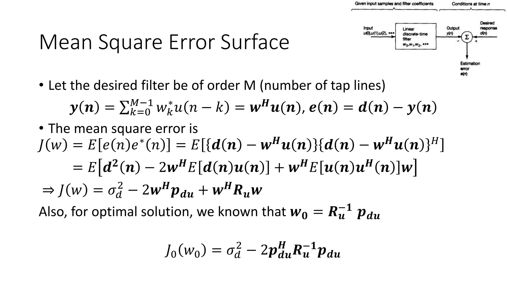
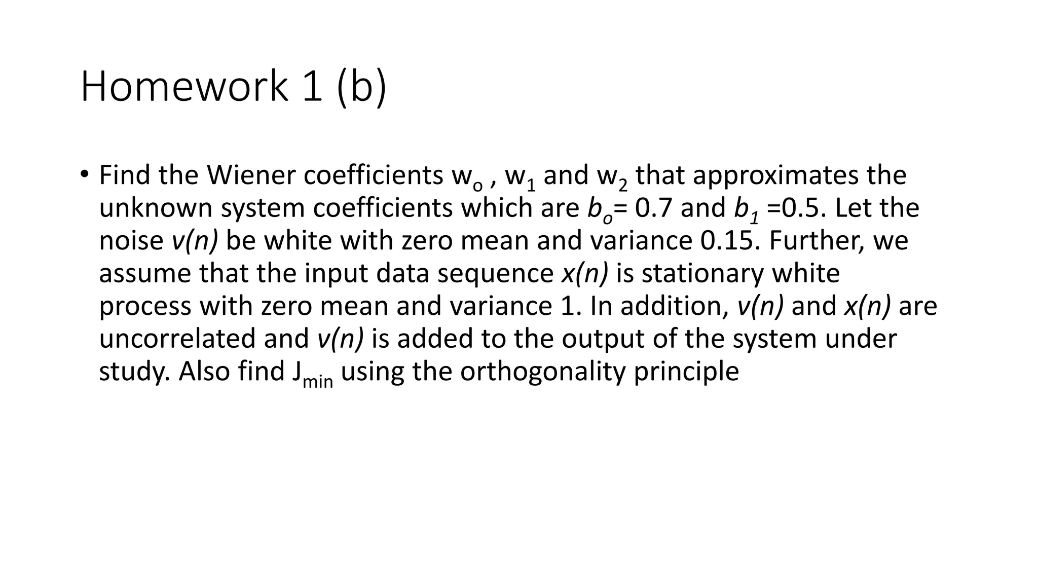
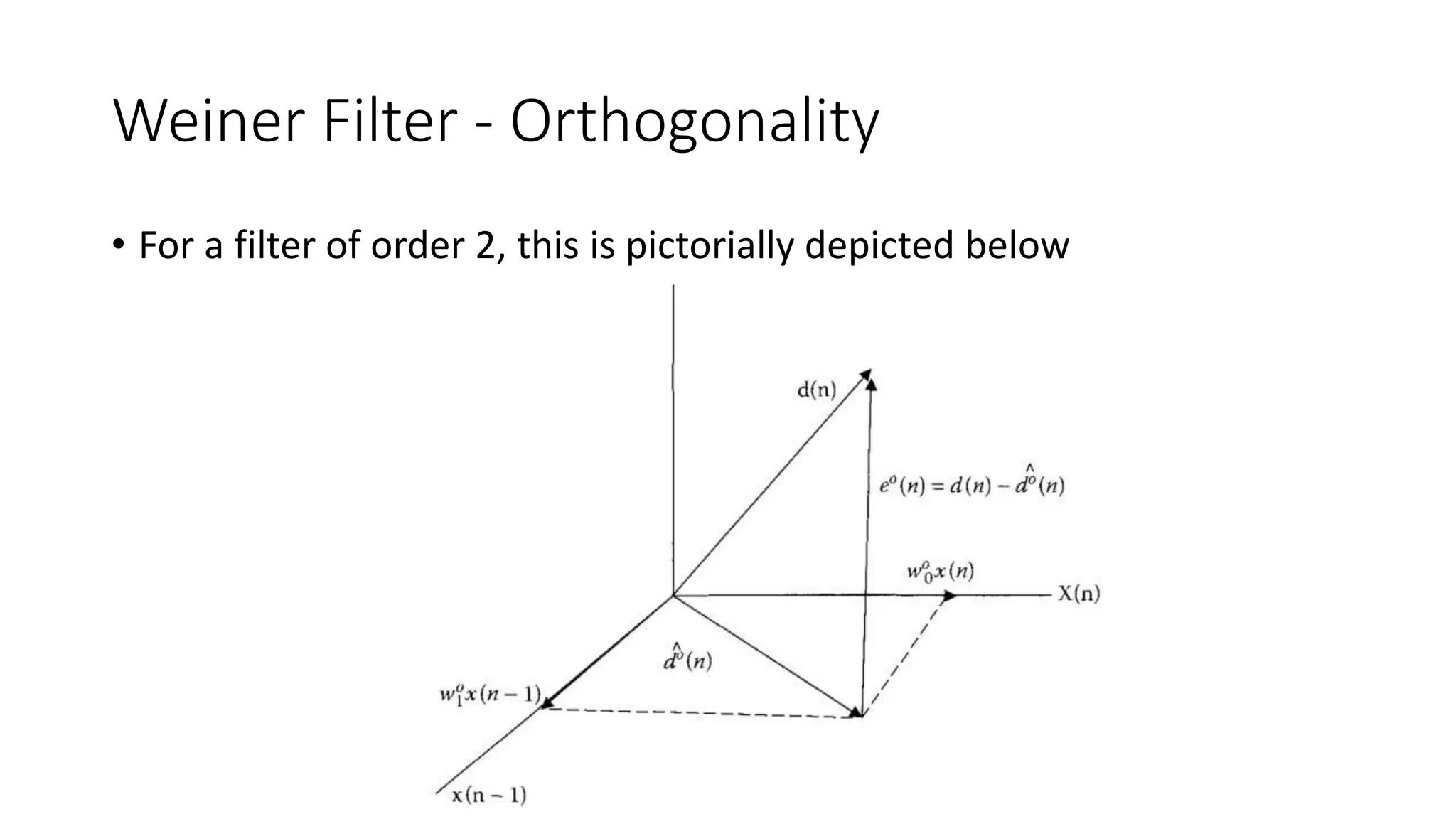
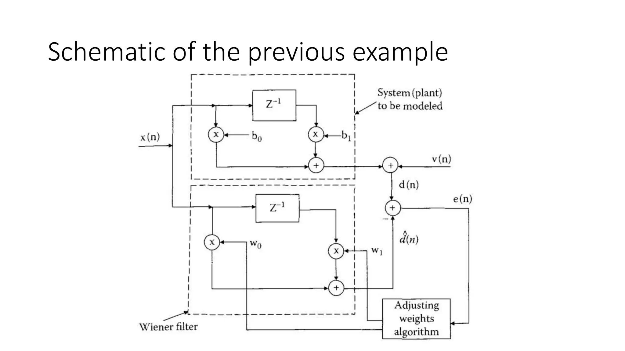
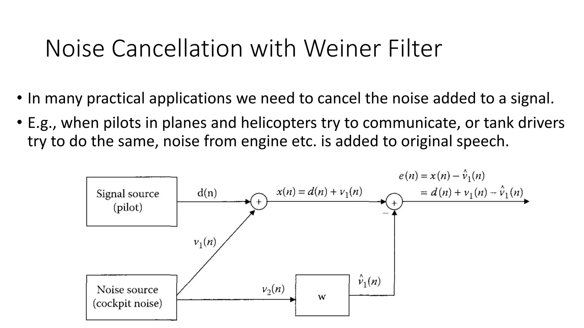
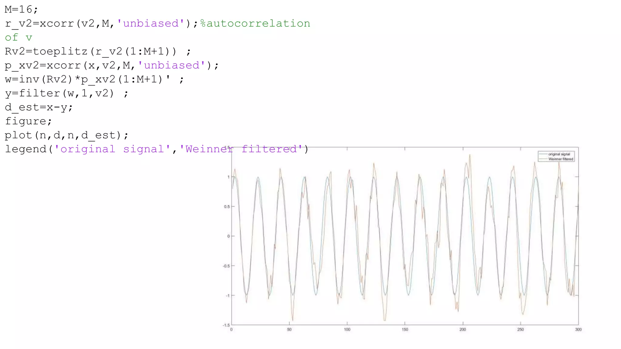
The document discusses the derivation and properties of Wiener filters, which are linear filters that minimize the mean square error between the desired signal and the estimate. Specifically: - It derives the Weiner-Hopf equation, which provides the condition for optimal filter weights to minimize the mean square error. - It shows that the optimal filter output and minimum error are orthogonal. - It discusses how the Weiner filter can be used for applications like noise cancellation by estimating the desired signal using two microphones. 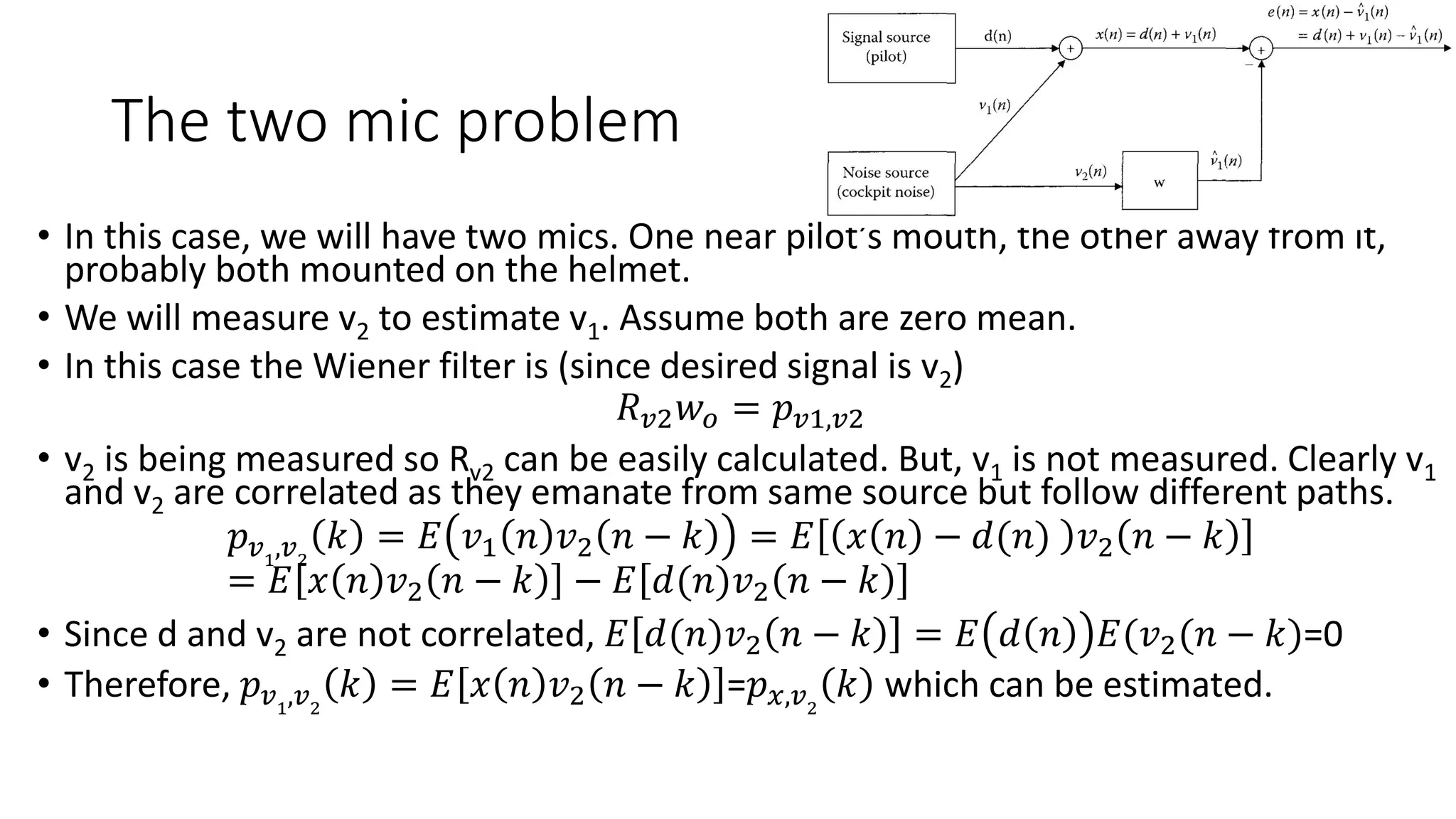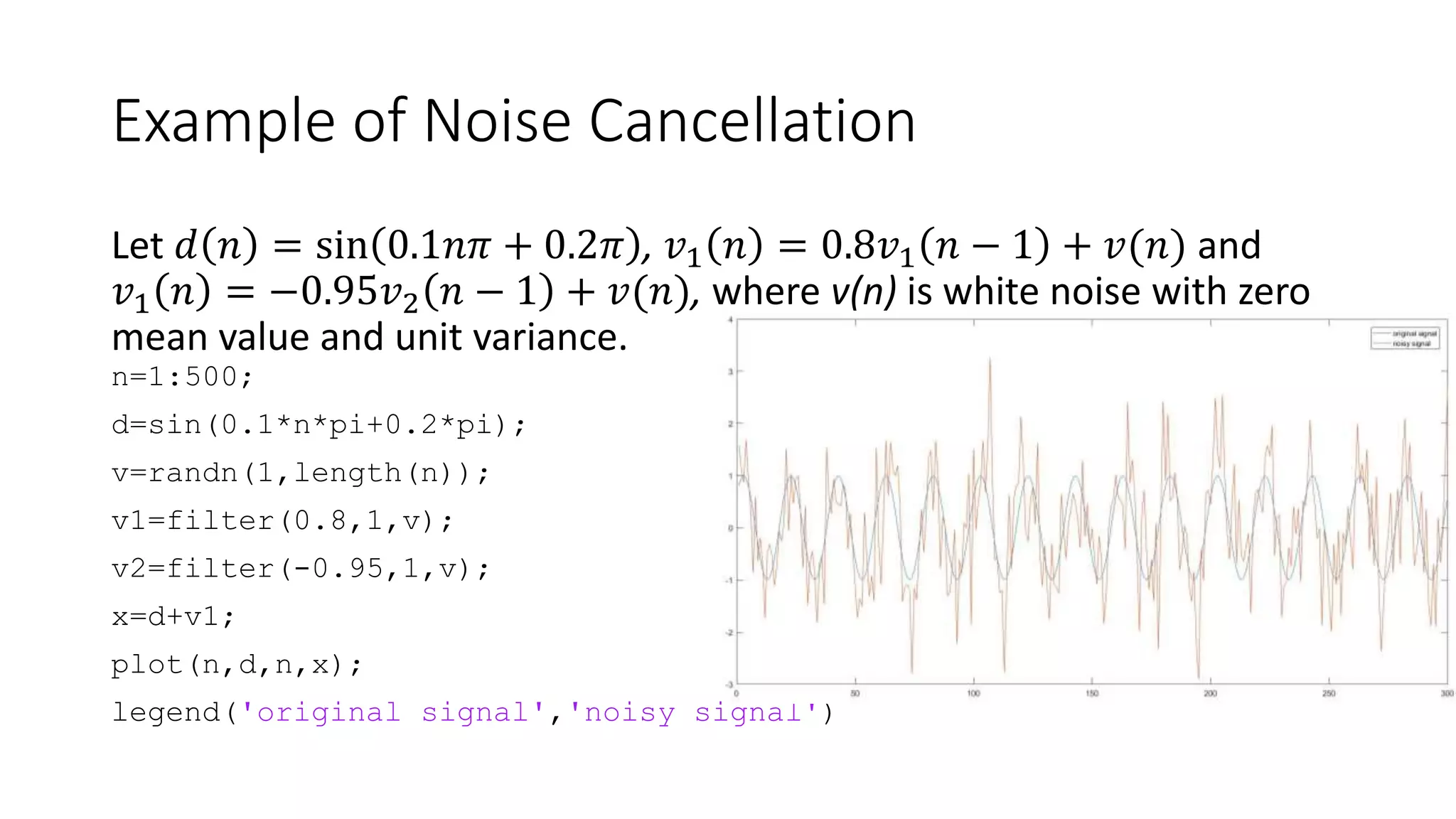- It provides an example of applying a Weiner filter to cancel noise from a signal measured by two microphones mounted on a pilot's helmet.

1. Av-738
Adaptive Filter Theory
Lecture 3- Optimum Filtering
[Weiner Filters]
Dr. Bilal A. Siddiqui
Air University (PAC Campus)
Spring 2018

2. Linear Optimum Filtering
• Consider a linear discrete-time filter
• The filter is linear (to make mathematical analysis easier to handle)
• Filter operates in discrete time (makes implementation easier)
• The requirement is to make the filter error e(n) as small as possible in some statistical sense
• Statistical “sense” means filter output should be optimum (minimizing some criteria). Candidate
criteria are expectation of:
• Absolute value of estimation error
• Square of absolute value (or mean-square value) of estimation error
• Third or higher power of absolute value of estimation error
• Option 1 has a discontinuous first derivative. Option 3 is also mathematically cumbersome
• Option 2 has a unique minimum, and has a second order dependence on filter weights, which
makes optimization possible.
𝐽 = 𝐸 𝑒 𝑛 𝑒∗ 𝑛 = 𝐸 𝑒 𝑛 2
• The linear optimal filtering problem is then formally stated as “design a discrete-time linear filter
whose output y(n) provides an estimate of the desired response d(n) such that mean-square value of
estimation error is minimized.”

3. Weiner filter – Derivation ,part 1
• The problem is to minimize J by choosing the optimum weights w0
• Since filter coefficients are also (in general complex), 𝑤 𝑘 = 𝑎 𝑘 + 𝑗𝑏 𝑘
• Let’s define the gradient operator (general derivative), 𝛻𝑘 =
𝜕
𝜕𝑎 𝑘
+ 𝑗
𝜕
𝜕𝑏 𝑘
• Multi-dimensional gradient of the (scalar and real) cost function is, therefore 𝛻𝑘 𝐽 =
𝜕𝐽
𝜕𝑎 𝑘
+ 𝑗
𝜕𝐽
𝜕𝑏 𝑘
• For J to attain a minimum, the necessary condition is 𝛻𝑘 𝐽 = 0
𝛻𝑘 𝐽 = 𝛻𝑘 𝐸 𝑒 𝑛 𝑒∗ 𝑛 = 𝐸 𝛻𝑘 𝑒 𝑛 𝑒∗ 𝑛
𝛻𝑘 𝐽 = 𝐸
𝜕𝑒 𝑛
𝜕𝑎 𝑘
𝑒∗
𝑛 +
𝜕𝑒∗
𝑛
𝜕𝑎 𝑘
𝑒 𝑛 + 𝑗
𝜕𝑒 𝑛
𝜕𝑏 𝑘
𝑒∗
𝑛 +
𝜕𝑒∗
𝑛
𝜕𝑏 𝑘
𝑒 𝑛

4. Weiner filter – derivation 2
𝛻𝑘 𝐽 = 𝐸
𝜕𝑒 𝑛
𝜕𝑎 𝑘
𝑒∗ 𝑛 +
𝜕𝑒∗ 𝑛
𝜕𝑎 𝑘
𝑒 𝑛 +
𝜕𝑒 𝑛
𝜕𝑏 𝑘
𝑗𝑒∗ 𝑛 +
𝜕𝑒∗ 𝑛
𝜕𝑏 𝑘
𝑗𝑒 𝑛
• Since, 𝑒 𝑛 = 𝑑 𝑛 − 𝑘=0
𝑀−1
𝑤 𝑘
∗
𝑢 𝑛 − 𝑘 = 𝑑 𝑛 + 𝑘=0
𝑀−1
−𝑎 𝑘 + 𝑗𝑏 𝑘 𝑢 𝑛 − 𝑘
and d(n) is not a function of wk
𝛻𝑘 𝐽 = −2𝐸 𝑢 𝑛 − 𝑘 𝑒∗
𝑛
• If e0 is the special value of estimation error when filter operates in optimum condition
𝐸 𝑢 𝑛 − 𝑘 𝑒0
∗
𝑛 = 0
• This is an optimum result. It states that, “The necessary and sufficient condition for the cost
function J to attain its minimum, the error value at the operating condition is orthogonal (i.e.
unaffected) by all the samples of input used to calculate that estimate.”
• Since 𝐸 𝑦 𝑛 𝑒∗
𝑛 = 𝐸 𝑘=0
𝑀−1
𝑤 𝑘
∗
𝑢 𝑛 − 𝑘 𝑒∗
𝑛 = 𝑘=0
𝑀−1
𝑤 𝑘
∗
𝐸 𝑢 𝑛 − 𝑘 𝑒∗
𝑛
• This means 𝐸 𝑦0 𝑛 𝑒0
∗
𝑛 = 0, i.e. optimum output is orthogonal to min. error

5. Weiner Filter - Orthogonality
• For a filter of order 2, this is pictorially depicted below

6. Weiner-Hopf Equation
• Let’s re-write the orthogonality condition in terms of optimal weights (k=0,1,2,…M-1)
𝐸 𝑢 𝑛 − 𝑘 𝑒0
∗
𝑛 = 𝐸 𝑢 𝑛 − 𝑘 𝑑∗
−
𝑙=0
𝑀−1
𝑤𝑙,0 𝑢∗
𝑛 − 𝑙 = 0
Expanding the equation for
𝑙=0
𝑀−1
𝑤𝑙,0 𝐸 𝑢 𝑛 − 𝑘 𝑢∗
𝑛 − 𝑙 = 𝐸 𝑢 𝑛 − 𝑘 𝑑∗
𝑛
Recognizing autocorrelation 𝑟 𝑙 − 𝑘 = 𝐸 𝑢 𝑛 − 𝑘 𝑢∗ 𝑛 − 𝑙 and cross-correlation 𝑝 −𝑘 = 𝐸 𝑢 𝑛 − 𝑘 𝑑∗ 𝑛
𝑙=0
𝑀−1
𝑤𝑙,0 𝑟 𝑙 − 𝑘 = 𝑝 −𝑘
This can be written in matrix form for 𝑢 𝑛 = [𝑢 𝑛 𝑢 𝑛 − 1 … 𝑢 𝑛 − 𝑀 − 1 ], 𝑹 𝒖 = 𝐸 𝑢 𝑛 𝑢 𝐻
𝑛 ,
𝒑 𝒅𝒖 = 𝑝 0 𝑝 1 … 𝑝 𝑀 − 1 and 𝒘 𝟎 = 𝑤0,0 𝑤1,0 … 𝑤 𝑀−1,0
𝒘 𝟎 = 𝑹 𝒖
−𝟏
𝒑 𝒅𝒖
This is known as the Weiner-Hopf equation

7. Mean Square Error Surface
• Let the desired filter be of order M (number of tap lines)
𝒚 𝒏 = 𝑘=0
𝑀−1
𝑤 𝑘
∗
𝑢 𝑛 − 𝑘 = 𝒘 𝑯 𝒖(𝒏), 𝒆 𝒏 = 𝒅 𝒏 − 𝒚 𝒏
• The mean square error is
𝐽 𝑤 = 𝐸 𝑒 𝑛 𝑒∗
𝑛 = 𝐸 𝒅 𝒏 − 𝒘 𝑯
𝒖 𝒏 𝒅 𝒏 − 𝒘 𝑯
𝒖 𝒏 𝐻
= 𝐸 𝒅 𝟐
𝒏 − 2𝒘 𝑯
𝐸 𝒅 𝒏 𝒖 𝒏 + 𝒘 𝑯
𝐸 𝒖 𝒏 𝒖 𝑯
𝒏 𝒘
⇒ 𝐽 𝑤 = 𝜎 𝑑
2
− 2𝒘 𝑯
𝒑 𝒅𝒖 + 𝒘 𝑯
𝑹 𝒖 𝒘
Also, for optimal solution, we known that 𝒘 𝟎 = 𝑹 𝒖
−𝟏 𝒑 𝒅𝒖
𝐽0 𝑤0 = 𝜎 𝑑
2
− 2𝒑 𝒅𝒖
𝑯
𝑹 𝒖
−𝟏
𝒑 𝒅𝒖

8. Example: System Identification
• Find the optimum filter coefficients wo and w1 of the Wiener filter,
which approximates (models) the unknown FIR system with
coefficients bo= 1.5 and b1= 0.5 and contaminated with additive white
uniformly distributed noise of 0.02 variance. Input is white Gaussian
noise of variance 1.
clc;clear;
n =0.5*(rand(1,200)-0.5);%n=noise vector with zero mean and variance 0.02
u=randn(1,200);% u=data vector entering the system
y=filter( [1.5 0.5],1,u); %filter output
d=y + n; % desired output
[ru,lagsru]=xcorr(u,1,'unbiased') ;
Ru=toeplitz(ru(1:2));
[pdu,lagsdu]=xcorr(u,d,1,'unbiased') ;
W_opt=inv(Ru) *pdu(1:2)' ; % optimum Weiner filter weights
sigma2d=xcorr(d,d,0);%autocorrelation of d at zero lag
jmin=mean((d-filter(w_opt,1,u)).^2);

9. Error Surface
w=[linspace(-3*w_opt(1),3*w_opt(1),50);linspace(-9*w_opt(2),9*w_opt(2),50)];
[w1,w2]=meshgrid(w(1,:),w(2,:));
for k=1:length(w1)
for l=1:length(w2)
J(k,l)=mean((d-filter([w1(k,l) w2(k,l)],1,u)).^2);
end
end
surf(w1,w2,J);
xlabel('W_1');ylabel('W_2');zlabel('Cost Function, J');

10. Schematic of the previous example

11. Noise Cancellation with Weiner Filter
• In many practical applications we need to cancel the noise added to a signal.
• E.g., when pilots in planes and helicopters try to communicate, or tank drivers
try to do the same, noise from engine etc. is added to original speech.

12. The two mic problem
• In this case, we will have two mics. One near pilot’s mouth, the other away from it,
probably both mounted on the helmet.
• We will measure v2 to estimate v1. Assume both are zero mean.
• In this case the Wiener filter is (since desired signal is v2)
𝑅 𝑣2 𝑤𝑜 = 𝑝 𝑣1,𝑣2
• v2 is being measured so Rv2 can be easily calculated. But, v1 is not measured. Clearly v1
and v2 are correlated as they emanate from same source but follow different paths.
𝑝 𝑣1
,𝑣2
𝑘 = 𝐸 𝑣1 𝑛 𝑣2 𝑛 − 𝑘 = 𝐸 𝑥 𝑛 − 𝑑(𝑛) 𝑣2 𝑛 − 𝑘
= 𝐸 𝑥 𝑛 𝑣2 𝑛 − 𝑘 − 𝐸 𝑑(𝑛)𝑣2 𝑛 − 𝑘
• Since d and v2 are not correlated, 𝐸 𝑑(𝑛)𝑣2 𝑛 − 𝑘 = 𝐸 𝑑 𝑛 𝐸(𝑣2(𝑛 − 𝑘)=0
• Therefore, 𝑝 𝑣1
,𝑣2
𝑘 = 𝐸 𝑥 𝑛 𝑣2 𝑛 − 𝑘 =𝑝 𝑥,𝑣2
𝑘 which can be estimated.

13. Example of Noise Cancellation
Let 𝑑 𝑛 = sin 0.1𝑛𝜋 + 0.2𝜋 , 𝑣1 𝑛 = 0.8𝑣1 𝑛 − 1 + 𝑣(𝑛) and
𝑣1 𝑛 = −0.95𝑣2 𝑛 − 1 + 𝑣(𝑛), where v(n) is white noise with zero
mean value and unit variance.
n=1:500;
d=sin(0.1*n*pi+0.2*pi);
v=randn(1,length(n));
v1=filter(0.8,1,v);
v2=filter(-0.95,1,v);
x=d+v1;
plot(n,d,n,x);
legend('original signal','noisy signal')

14. M=16;
r_v2=xcorr(v2,M,'unbiased');%autocorrelation
of v
Rv2=toeplitz(r_v2(1:M+1)) ;
p_xv2=xcorr(x,v2,M,'unbiased');
w=inv(Rv2)*p_xv2(1:M+1)' ;
y=filter(w,1,v2) ;
d_est=x-y;
figure;
plot(n,d,n,d_est);
legend('original signal','Weinner filtered')

15. Homework 1 (b)
• Find the Wiener coefficients wo , w1 and w2 that approximates the
unknown system coefficients which are bo= 0.7 and b1 =0.5. Let the
noise v(n) be white with zero mean and variance 0.15. Further, we
assume that the input data sequence x(n) is stationary white
process with zero mean and variance 1. In addition, v(n) and x(n) are
uncorrelated and v(n) is added to the output of the system under
study. Also find Jmin using the orthogonality principle