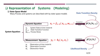
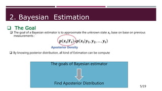
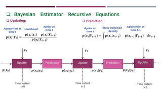
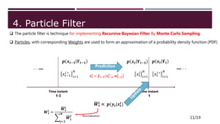
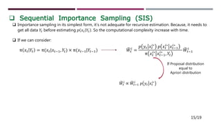
This document provides an overview of particle filtering and sampling algorithms. It discusses key concepts like Bayesian estimation, Monte Carlo integration methods, the particle filter, and sampling algorithms. The particle filter approximates probabilities with weighted samples to estimate states in nonlinear, non-Gaussian systems. It performs recursive Bayesian filtering by predicting particle states and updating their weights based on new observations. While powerful, particle filters have high computational complexity and it can be difficult to determine the optimal number of particles.

1. IN THE NAME OF GOD
Title:
Particle Filter and Sampling
Algorithms
By:
Mohammad Reza Jabbari
Email: Mo.re.jabbari@gmail.com

2. Outline
1. Estimation Concepts
2. Bayesian Estimation
3. Monte Carlo Integration Methods
4. Particle Filter
5. Sampling Algorithms
6. Application
7. Summery
8. End
2/182/19

3. 1.Estimation Concepts
 The purpose of estimation is to obtain an Approximate Value of an Unknown Parameter, based on
Noisy Observations made from measurements.
Estimation
Theory
Classic
(Estimation of a Parameter)
Bayesian
(Estimation of a Random Variable)
Point Estimation
Interval Estimation
Method of Moment
Maximum Likelihood (ML)
Kalman Filter (KF)
Extended Kalman Filter (EKF)
Unscented Kalman Filter (UKF)
Particle Filter (PF)
Linearity / Gaussian
low nonlinearity / Gaussian
high nonlinearity / Gaussian
Recursive
form
nonlinearity / non Gaussian
 Definition And Classification
3/183/19

4. 4/18
 Representation of Systems (Modeling)
 State-Space Model
Many Process and systems can described with by state-space models
System Equation:
Dynamic Equation
Measurement Equation 𝒚 𝒕 = 𝒉 𝒕 𝒙 𝒕, 𝒗 𝒕
𝒙 𝒕 = 𝒇 𝒕−𝟏 𝒙 𝒕−𝟏, 𝒘 𝒕−𝟏
𝒙 𝒕 System State at time instant t
𝒇 𝒕−𝟏 State Transition Function
𝒘 𝒕−𝟏 Process Noise
𝒚𝒕 Observation at time instant t
𝒉 𝒕 Observation Function
𝒗 𝒕 Obseravtion Noise
𝒑(𝒙 𝒕|𝒙 𝒕−𝟏)
𝒑 𝒚 𝒕 𝒙 𝒕
Probabilistic
form
Probabilistic
form
Likelihood Density
State Transition Density
4/19

5. 2. Bayesian Estimation
 The Goal
 The goal of a Bayesian estimator is to approximate the unknown state 𝒙 𝒕 base on base on previous
measurements :
𝒑 𝒙 𝒕 𝒀 𝒕 = 𝒑 𝒙 𝒕 𝒚 𝟏, 𝒚 𝟐, … , 𝒚 𝒕
Aposterior Density
 By knowing posterior distribution, all kind of Estimation can be compute
The goals of Bayesian estimator
Find Aposterior Distribution
5/19

6. 6/18
 Bayesian Estimator Recursive Equations
 Updating:  Prediction:
𝒑 𝒙 𝒕 𝒀 𝒕 =
𝒑 𝒚 𝒕 𝒙 𝒕 𝒑 𝒙 𝒕 𝒀 𝒕−𝟏
𝒑 𝒚 𝒕 𝒀 𝒕−𝟏
𝒑 𝒙 𝒕 𝒀 𝒕−𝟏 = 𝒑 𝒙 𝒕 𝒙 𝒕−𝟏 𝒑 𝒙 𝒕−𝟏 𝒀 𝒕−𝟏 𝒅𝒙 𝒕−𝟏
State transition
density
Aprior at
time t
Aposteriori at
time t-1Aposteriori at
time t
Aprior at
time tLikelihood
𝒑 𝒙 𝟎 𝒚 𝟎 𝒑 𝒙 𝟏 𝒚 𝟎 𝒑 𝒙 𝟏 𝒚 𝟏 𝒑 𝒙 𝟐 𝒚 𝟏
Prediction PredictionUpdate Update Update
𝒑(𝒙 𝟎)
𝒚 𝟎 𝒚 𝟏 𝒚 𝟐
Time instant
t=0
Time instant
t=1
Time instant
t=2

7. 7/18
 Problems
 The solution is conceptual because integral are not tractable
 Close form solution are possible in a small number of situation
 Solution
 Use Monte Carlo Integration Methods
For linear systems with Gaussian noise distribution
Optimal Estimation Using the Kalman Filter (KF)
7/19

8. 3. Monte Carlo Integration Methods
 Monte Carlo Integration is a Simple but Powerful technique for approximating complicated integrals.
 Assume we are trying to estimate the integral of a function f over some domain D :
Assume that we have a PDF p defined over a domain D :
Its means that we generate samples according to p, computing f/p for each sample, and finding the
average of these values.
 This equality is true for any PDF on D, as long as p(x)≠0 whenever f(x)≠0
9/19

9. 9/18
 Question
 What happens when we generate a random sample where the value of p is very small?
if p is very small for a given sample, f/p will be arbitrarily large. This large sample will greatly skew
the sample mean away from the true mean, and the sample variance will also increase greatly.
Bad Samples
 but one general rule of thumb to follow is that p should “look like” f (Importance Sampling)
 Answer
10/19

10. 4. Particle Filter
 The particle filter is technique for implementing Recursive Bayesian Filter By Monte Carlo Sampling
 Particles, with corresponding Weights are used to form an approximation of a probability density function (PDF)
𝑥𝑡−1
𝑖 ∗
𝑖=1
𝑁
𝑥𝑡
𝑖
𝑖=1
𝑁
𝑥𝑡
𝑖 ∗
𝑖=1
𝑁
Time instant
t-1
Time instant
t
𝒑 𝒙 𝒕−𝟏 𝒀 𝒕−𝟏 𝒑 𝒙 𝒕 𝒀 𝒕−𝟏 𝒑 𝒙 𝒕 𝒀 𝒕
Prediction
𝒙 𝒕
𝒊
= 𝒇 𝒕−𝟏(𝒙 𝒕−𝟏
𝒊 ∗
, 𝒘 𝒕−𝟏
𝒊
𝑾 𝒕
𝒊
∝ 𝒑(𝒚 𝒕|𝒙 𝒕
𝒊
)
𝑾 𝒕
𝒊
=
𝑾 𝒕
𝒊
𝒋=𝟏
𝑵
𝑾 𝒕
𝒋 Normalization
11/19

11. 11/18
 Sample Representation of the posterior pdf
 The representation of the posterior pdf in the form of a set of samples is very convenient
For example: threat analysis, decision and control problems,
𝐸 𝐶 𝑥𝑡 𝑌𝑡 = 𝐶 𝑥𝑡 𝑝 𝑥𝑡 𝑌𝑡 𝑑𝑥𝑡 ≈
𝑖=1
𝑁
𝑊𝑡
𝑖
𝐶(𝑥𝑡
𝑖
) ≈
1
𝑁
𝑖=1
𝑁
𝐶(𝑥𝑡
𝑖∗
 In many cases, the requirement is find some particular function of the posterior, and the sample
representation is often ideal for this.
𝑝(𝑥 𝑡|𝑌𝑡−1) ≈
1
𝑁
𝑖=1
𝑁
𝛿 (𝑥 𝑡 − 𝑥 𝑡
𝑖
)
𝑝(𝑥 𝑡|𝑌𝑡) ≈
𝑖=1
𝑁
𝑊𝑡
𝑖
𝛿 (𝑥 𝑡 − 𝑥 𝑡
𝑖
) ≈
1
𝑁
𝑖=1
𝑁
𝛿 (𝑥 𝑡 − 𝑥 𝑡
𝑖∗
)
Empirical Distribution
12/19

12. 12/18
 Unfortunately, it’s usually impossible to sample efficiently from the posteriori distribution at any time t,
because being multivariate , non standard and only known up to a proportionality constant.
 Importance Sampling
 Generate sample from another distribution (Proposal Distribution)
 Weight them according to how they fit the Posterior distribution
 Notice: Free to choose proposal density but:
 It should be easy to sample from proposal density
 Proposal density should resemble the original density as closely as possible
 Problem
 Solution
13/19

13. 5. Sampling Algorithms
 Importance Sampling (IS)
𝐸 𝐶 𝑥𝑡 𝑌𝑡 = 𝐶 𝑥𝑡 𝑝 𝑥𝑡 𝑌𝑡 𝑑𝑥𝑡 ≈ 𝐶 𝑥𝑡
𝑝 𝑥𝑡 𝑌𝑡
π(𝑥𝑡|𝑌𝑡)
π(𝑥𝑡|𝑌𝑡) 𝑑𝑥𝑡 ≈
1
𝑁
𝑖=1
𝑁
𝐶(𝑥𝑡
𝑖∗
)
𝑝 𝑥𝑡
𝑖∗
𝑌𝑡
π(𝑥𝑡
𝑖∗
|𝑌𝑡)
Importance
Weight
𝑝 𝑌𝑡 𝑥𝑡
𝑖∗
𝑝(𝑥𝑡
𝑖∗
π(𝑥 𝑡
𝑖∗
|𝑌𝑡
14/19

14. 14/18
 Sequential Importance Sampling (SIS)
 Importance sampling in its simplest form, it’s not adequate for recursive estimation. Because, it needs to
get all data 𝑌𝑡 before estimating 𝑝 𝑥 𝑡 𝑌𝑡 . So the computational complexity increase with time.
π 𝑥𝑡 𝑌𝑡 = π(𝑥𝑡|𝑥𝑡−1, 𝑌𝑡) × π(𝑥𝑡−1|𝑌𝑡−1)
 If we can consider:
𝑊𝑡
𝑖
=
𝑝 𝑦𝑡 𝑥𝑡
𝑖∗
𝑝 𝑥𝑡
𝑖∗
𝑥𝑡−1
𝑖∗
π 𝑥𝑡
𝑖∗
𝑥𝑡−1
𝑖∗
, 𝑌𝑡
𝑊𝑡−1
𝑖
𝑊𝑡
𝑖
∝ 𝑊𝑡−1
𝑖
𝑝 𝑦𝑡 𝑥 𝑡
𝑖∗
If Proposal distribution
equal to
Apriori distribution
15/19

15. 15/18
 Sequential Importance Resampling (SIR)
 Problem:
The problem encountered by the SIS
method is that, as t increase, the
distribution of the importance weight
becomes more and more skewed. And
after a few time step, only one particle
has a non-zero importance weight.
(Degeneracy)
 Solution:
the key idea is to eliminate the
particles having low importance
weights and multiply particles having
high importance weigh
(Resampling)
16/19

16. 16/18
 Problem of Resampling
 Impoverishment of the sample set
particles with large weights may be selected many times so that the new set of samples may contain multiple
copies of just a few distinct values.
 Solution: Effective Sample Size
𝑁𝑒𝑓𝑓 =
1
𝑗=1
𝑁
𝑊𝑡
𝑗 2 𝑎𝑛𝑑 1 ≤ 𝑁𝑒𝑓𝑓 ≤ 𝑁
17/19

17. 6. Application
 Image Processing
 Sound Processing
 Tracking and Navigation
 Channel Estimation
 Biology
 ….
Base on image
1. Image Processing and Extract features
2. Estimation
18/19

18. 7. Summary
 Particle filter is very powerful framework for estimating parameter in nonlinear / non Gaussian model
 Adapting with state-space model
 Finding new application for particle filter
 Developing new implementation to reduce complexity
 Finding a mechanism to optimize number of particle
 Advantages
 Disadvantages
 High Computational Complexity
 It’s difficult to determine optimal Number of Particles
 Increasing particle with increasing model dimension
 Choice of importance density
 Main Research Directory
19/19

19. THE END