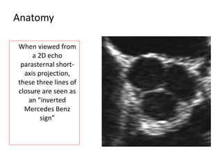
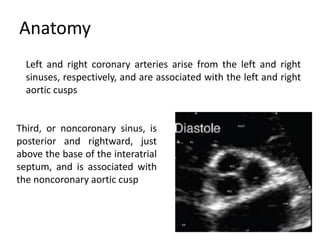
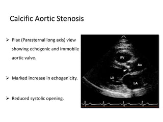
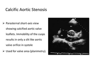
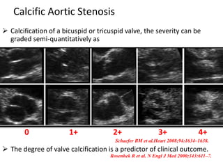
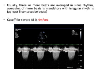
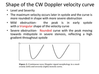
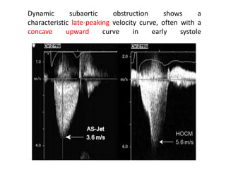
Three sentences:
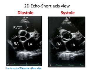
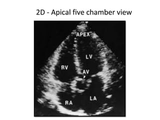
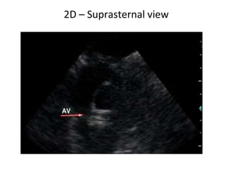
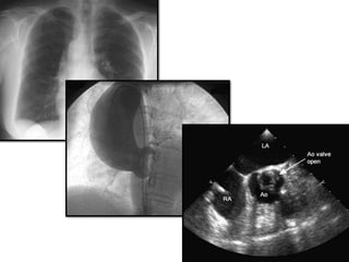
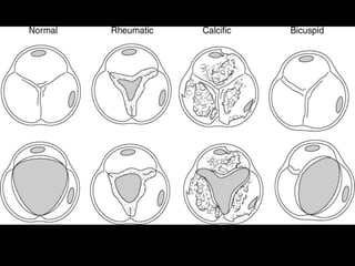
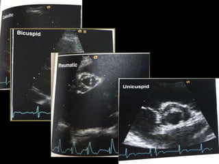
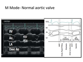
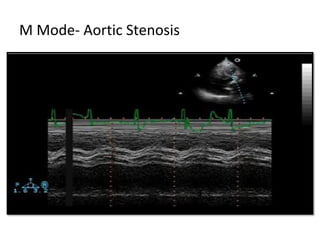
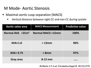
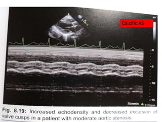
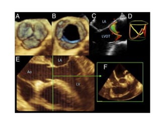
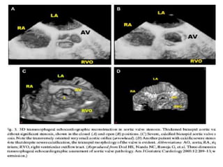
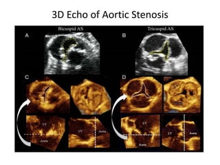
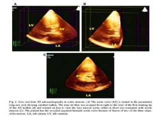
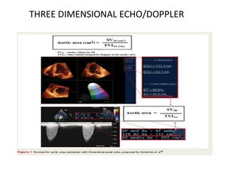
The document provides details on the anatomy and evaluation of aortic stenosis using echocardiography. It describes the normal aortic valve anatomy and how various types of aortic stenosis like calcific, rheumatic, bicuspid and subvalvular present on echo. Quantitative assessment of aortic stenosis severity is done using Doppler ultrasound to measure the maximum jet velocity and calculate the pressure gradient across the stenotic valve.
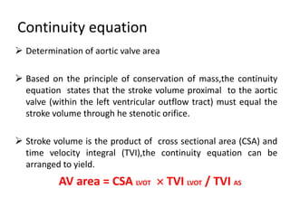
A lecture on the echocardiographic evaluation of hypertrophic cardiomyopathy. Starts with an overview of the topic then a systematic approach to diagnosis and then a differential diagnosis followed by take-home messages and conclusion.
preop TEE assessment of atrial septal defect is very important for making decision for device closure, properly assessed adequate rims of ASD will reduce risk of device embolization to almost nil.
Echo assesment of Aortic Stenosis and Regurgitationdrpraveen1986
A simple ppt presentation on echo assesment of AS and AR. Don forget to leave a comment if u find this ppt useful. - Dr. Praveen Babu, Vijaya HOspital, Chennai
Peter Hansen is a Cardiologist with a particular interest in Transcatheter Aortic Valve Implantation. This talk is all about TAVI's and imaging used to assess them. You may be seeing a lot more TAVI's so this superb insight from an expert is invaluable.
a cardiac surgery presentation about Atrioventricular septal defect,Definition, Prevalence,Anatomy,Classification,presentation ,diagnosis and management
New Directions in Targeted Therapeutic Approaches for Older Adults With Mantl...i3 Health
i3 Health is pleased to make the speaker slides from this activity available for use as a non-accredited self-study or teaching resource.
This slide deck presented by Dr. Kami Maddocks, Professor-Clinical in the Division of Hematology and
Associate Division Director for Ambulatory Operations
The Ohio State University Comprehensive Cancer Center, will provide insight into new directions in targeted therapeutic approaches for older adults with mantle cell lymphoma.
STATEMENT OF NEED
Mantle cell lymphoma (MCL) is a rare, aggressive B-cell non-Hodgkin lymphoma (NHL) accounting for 5% to 7% of all lymphomas. Its prognosis ranges from indolent disease that does not require treatment for years to very aggressive disease, which is associated with poor survival (Silkenstedt et al, 2021). Typically, MCL is diagnosed at advanced stage and in older patients who cannot tolerate intensive therapy (NCCN, 2022). Although recent advances have slightly increased remission rates, recurrence and relapse remain very common, leading to a median overall survival between 3 and 6 years (LLS, 2021). Though there are several effective options, progress is still needed towards establishing an accepted frontline approach for MCL (Castellino et al, 2022). Treatment selection and management of MCL are complicated by the heterogeneity of prognosis, advanced age and comorbidities of patients, and lack of an established standard approach for treatment, making it vital that clinicians be familiar with the latest research and advances in this area. In this activity chaired by Michael Wang, MD, Professor in the Department of Lymphoma & Myeloma at MD Anderson Cancer Center, expert faculty will discuss prognostic factors informing treatment, the promising results of recent trials in new therapeutic approaches, and the implications of treatment resistance in therapeutic selection for MCL.
Target Audience
Hematology/oncology fellows, attending faculty, and other health care professionals involved in the treatment of patients with mantle cell lymphoma (MCL).
Learning Objectives
1.) Identify clinical and biological prognostic factors that can guide treatment decision making for older adults with MCL
2.) Evaluate emerging data on targeted therapeutic approaches for treatment-naive and relapsed/refractory MCL and their applicability to older adults
3.) Assess mechanisms of resistance to targeted therapies for MCL and their implications for treatment selection
Title: Sense of Smell
Presenter: Dr. Faiza, Assistant Professor of Physiology
Qualifications:
MBBS (Best Graduate, AIMC Lahore)
FCPS Physiology
ICMT, CHPE, DHPE (STMU)
MPH (GC University, Faisalabad)
MBA (Virtual University of Pakistan)
Learning Objectives:
Describe the primary categories of smells and the concept of odor blindness.
Explain the structure and location of the olfactory membrane and mucosa, including the types and roles of cells involved in olfaction.
Describe the pathway and mechanisms of olfactory signal transmission from the olfactory receptors to the brain.
Illustrate the biochemical cascade triggered by odorant binding to olfactory receptors, including the role of G-proteins and second messengers in generating an action potential.
Identify different types of olfactory disorders such as anosmia, hyposmia, hyperosmia, and dysosmia, including their potential causes.
Key Topics:
Olfactory Genes:
3% of the human genome accounts for olfactory genes.
400 genes for odorant receptors.
Olfactory Membrane:
Located in the superior part of the nasal cavity.
Medially: Folds downward along the superior septum.
Laterally: Folds over the superior turbinate and upper surface of the middle turbinate.
Total surface area: 5-10 square centimeters.
Olfactory Mucosa:
Olfactory Cells: Bipolar nerve cells derived from the CNS (100 million), with 4-25 olfactory cilia per cell.
Sustentacular Cells: Produce mucus and maintain ionic and molecular environment.
Basal Cells: Replace worn-out olfactory cells with an average lifespan of 1-2 months.
Bowman’s Gland: Secretes mucus.
Stimulation of Olfactory Cells:
Odorant dissolves in mucus and attaches to receptors on olfactory cilia.
Involves a cascade effect through G-proteins and second messengers, leading to depolarization and action potential generation in the olfactory nerve.
Quality of a Good Odorant:
Small (3-20 Carbon atoms), volatile, water-soluble, and lipid-soluble.
Facilitated by odorant-binding proteins in mucus.
Membrane Potential and Action Potential:
Resting membrane potential: -55mV.
Action potential frequency in the olfactory nerve increases with odorant strength.
Adaptation Towards the Sense of Smell:
Rapid adaptation within the first second, with further slow adaptation.
Psychological adaptation greater than receptor adaptation, involving feedback inhibition from the central nervous system.
Primary Sensations of Smell:
Camphoraceous, Musky, Floral, Pepperminty, Ethereal, Pungent, Putrid.
Odor Detection Threshold:
Examples: Hydrogen sulfide (0.0005 ppm), Methyl-mercaptan (0.002 ppm).
Some toxic substances are odorless at lethal concentrations.
Characteristics of Smell:
Odor blindness for single substances due to lack of appropriate receptor protein.
Behavioral and emotional influences of smell.
Transmission of Olfactory Signals:
From olfactory cells to glomeruli in the olfactory bulb, involving lateral inhibition.
Primitive, less old, and new olfactory systems with different path
Ozempic: Preoperative Management of Patients on GLP-1 Receptor Agonists Saeid Safari
Preoperative Management of Patients on GLP-1 Receptor Agonists like Ozempic and Semiglutide
ASA GUIDELINE
NYSORA Guideline
2 Case Reports of Gastric Ultrasound
Flu Vaccine Alert in Bangalore Karnatakaaddon Scans
As flu season approaches, health officials in Bangalore, Karnataka, are urging residents to get their flu vaccinations. The seasonal flu, while common, can lead to severe health complications, particularly for vulnerable populations such as young children, the elderly, and those with underlying health conditions.
Dr. Vidisha Kumari, a leading epidemiologist in Bangalore, emphasizes the importance of getting vaccinated. "The flu vaccine is our best defense against the influenza virus. It not only protects individuals but also helps prevent the spread of the virus in our communities," he says.
This year, the flu season is expected to coincide with a potential increase in other respiratory illnesses. The Karnataka Health Department has launched an awareness campaign highlighting the significance of flu vaccinations. They have set up multiple vaccination centers across Bangalore, making it convenient for residents to receive their shots.
To encourage widespread vaccination, the government is also collaborating with local schools, workplaces, and community centers to facilitate vaccination drives. Special attention is being given to ensuring that the vaccine is accessible to all, including marginalized communities who may have limited access to healthcare.
Residents are reminded that the flu vaccine is safe and effective. Common side effects are mild and may include soreness at the injection site, mild fever, or muscle aches. These side effects are generally short-lived and far less severe than the flu itself.
Healthcare providers are also stressing the importance of continuing COVID-19 precautions. Wearing masks, practicing good hand hygiene, and maintaining social distancing are still crucial, especially in crowded places.
Protect yourself and your loved ones by getting vaccinated. Together, we can help keep Bangalore healthy and safe this flu season. For more information on vaccination centers and schedules, residents can visit the Karnataka Health Department’s official website or follow their social media pages.
Stay informed, stay safe, and get your flu shot today!
Knee anatomy and clinical tests 2024.pdfvimalpl1234
This includes all relevant anatomy and clinical tests compiled from standard textbooks, Campbell,netter etc..It is comprehensive and best suited for orthopaedicians and orthopaedic residents.
New Drug Discovery and Development .....NEHA GUPTA
The "New Drug Discovery and Development" process involves the identification, design, testing, and manufacturing of novel pharmaceutical compounds with the aim of introducing new and improved treatments for various medical conditions. This comprehensive endeavor encompasses various stages, including target identification, preclinical studies, clinical trials, regulatory approval, and post-market surveillance. It involves multidisciplinary collaboration among scientists, researchers, clinicians, regulatory experts, and pharmaceutical companies to bring innovative therapies to market and address unmet medical needs.
Couples presenting to the infertility clinic- Do they really have infertility...Sujoy Dasgupta
Dr Sujoy Dasgupta presented the study on "Couples presenting to the infertility clinic- Do they really have infertility? – The unexplored stories of non-consummation" in the 13th Congress of the Asia Pacific Initiative on Reproduction (ASPIRE 2024) at Manila on 24 May, 2024.
TEST BANK for Operations Management, 14th Edition by William J. Stevenson, Ve...kevinkariuki227
TEST BANK for Operations Management, 14th Edition by William J. Stevenson, Verified Chapters 1 - 19, Complete Newest Version.pdf
ARTIFICIAL INTELLIGENCE IN HEALTHCARE.pdfAnujkumaranit
Artificial intelligence (AI) refers to the simulation of human intelligence processes by machines, especially computer systems. It encompasses tasks such as learning, reasoning, problem-solving, perception, and language understanding. AI technologies are revolutionizing various fields, from healthcare to finance, by enabling machines to perform tasks that typically require human intelligence.
2. Anatomy
Aortic valve is composed of three cusps of equal size, each of
which is surrounded by a sinus
Cusps are separated by three commissures and supported by
a fibrous anulus
Each cusp is crescent shaped and capable of opening fully to
allow unimpeded forward flow, then closing tightly to prevent
regurgitation
4. Anatomy
Free edge of each cusp curves upward from the commissure
and forms a slight thickening at the tip or midpoint, called the
Arantius nodule
When the valve closes, the three nodes meet in the center,
allowing coaptation to occur along three lines that radiate out
from this center point
Overlap of valve tissue along the lines of closure produces a
tight seal and prevents backflow during diastole
5. Anatomy
When viewed from
a 2D echo
parasternal short-
axis projection,
these three lines of
closure are seen as
an “inverted
Mercedes Benz
sign”
6. Anatomy
• Behind each cusp is its associated Valsalva sinus
• Sinuses represent outpunching in the aortic root directly
behind each cusp
• Function to support the cusps during systole and provide a
reservoir of blood to augment coronary artery flow during
diastole
7. Anatomy
Left and right coronary arteries arise from the left and right
sinuses, respectively, and are associated with the left and right
aortic cusps
Third, or noncoronary sinus, is
posterior and rightward, just
above the base of the interatrial
septum, and is associated with
the noncoronary aortic cusp
RCC
LCC
NCC
LA
LAA
RA
RVOT
RV
8. Anatomy
The area of a normal aortic valve is 3 to 4 cm2
Normal opening generally produces 2 cm of
leaflet separation
Maintained throughout the cardiac cycle until low
cardiac output or LVOT obstruction
9. Goals of Echo
Establishing the diagnosis
Quantifying severity
Assessing left ventricular function
Identify concomitant valvular abnormalities
10. Role of 2D Echo
Visualizes the entire aortic valve structure
Helpful in identifying noncalcific as well as calcific aortic
stenosis
Degree of valvular calcification, the size of the aortic
anulus and the supravalvular ascending aorta, and the
presence of secondary subvalvular obstruction are easily
evaluated
Useful for determining the degree of LV hypertrophy
(wall thickness and mass), LA enlargement, ventricular
function, and the integrity of the other valves
11. Role of 2D Echo
Cusps are thickened and showed restricted mobility
Their position during systole is no longer parallel to the aortic
walls, and the edges are often seen to point toward the center
of the aorta
In severe cases, a nearly total lack of mobility may be present
and the anatomy may become so distorted that identification
of the individual cusps is impossible
16. Aortic Valve
Acquired valvular aortic stenosis – cusps become thickened,
restricted.
Position during systole is no longer parallel to the aortic walls.
Edges point toward the center of the aorta.
Severe cases – total lack of mobility. identification of cusps
may be impossible.
19. Aortic sclerosis
About 25% of all adults over age 65 yrs have aortic valve sclerosis.
Thickened calcified cusps with preserved mobility.
No significant obstruction to LV outflow.
Typically associated with peak doppler velocity of < 2.5 m/sec
In Cardiovascular Health Study ,for group of patients 65 yrs,the aortic
valve was normal in 70% of cases, sclerotic in 29% and stenotic in 2%
(JACC.1997;29(3))
In Euro Heart Survey of 4910 pts in 25 countries,AS was the most frequent
lesion,accounting for 43% of patients with VHD (Eur Heart J.2003;24(13):1231-43)
20. Calcific Aortic Stenosis
10-15% of aortic sclerosis patients progress to severe AS.
Nodular calcific masses on aortic side of cusps.
No commissural fusion.
Free edges of cusps are not involved.
Stellate- shaped systolic orifice
Cosmi et al,Arch Int Med 2002;162(20):2345-7.
21. Calcific Aortic Stenosis
Plax (Parasternal long axis) view
showing echogenic and immobile
aortic valve.
Marked increase in echogenicity.
Reduced systolic opening.
22. Calcific Aortic Stenosis
Parasternal short-axis view
showing calcified aortic valve
leaflets. Immobility of the cusps
results in only a slit like aortic
valve orifice in systole
Used for valve area (planimetry).
23. Calcific Aortic Stenosis
Calcification of a bicuspid or tricuspid valve, the severity can be
graded semi-quantitatively as
0 1+ 2+ 3+ 4+
Schaefer BM et al.Heart 2008;94:1634–1638.
The degree of valve calcification is a predictor of clinical outcome.
Rosenhek R et al. N Engl J Med 2000;343:611–7.
24. Directly planimetered aortic valve areas should be interpreted
with caution because of the complex anatomy of the orifice and
calcific shadowing and reverberation, even with 3D imaging.
Direct measurement of valve area on imaging reflects anatomic
valve area, whereas the doppler data provide functional area.
26. Bicuspid Aortic Valve (BAV)
Accounts for 2/3rd of cases of severe AS in adults < 70 yrs.
1/3rd of cases in adults > 70 yrs of age.
Severe AS of a BAV is difficult to be differentiated from that of tricuspid
one.
Usual view for differentiation is PARASTERNAL SHORT AXIS VIEW at
the level of great vessels in systole.
PARASTERNAL Long axis view shows systolic bowing of the leaflets into
aorta – “Dome like”.
M MODE – Eccentric closure line (to be taken at the tips of bowed
leaflets).
27. Bicuspid Aortic valve
Two cusps are seen in systole with only two commissures framing an
elliptical systolic orifice (the fish mouth appearance).
Diastolic images may mimic a tricuspid valve when a raphe is
present.
28. Bicuspid Aortic valve
In children, valve may be stenotic
without extensive calcification.
In adults, stenosis typically is due to
calcific changes, which often obscures
the number of cusps, making
determination of bicuspid vs. tricuspid
valve difficult.
33. Types of BAV
FUSION OF CUSPS FREQUENCY LEAFLET
CLOSURE LINE
REMARKS
RIGHT AND LEFT 70 -80% Anterolateral –
posteromedial closure
line
Larger anterior
leaflet.
RIGHT AND
NONCORONARY
20-30% Anterior –posterior
closure line
Larger rightward
leaflet
LEFT AND
NONCORONARY
1-2% Medial – lateral closure
line
Many bicuspid aortic valves have a raphe in the larger leaflet.
Clear identification of number of leaflets is possible only in systole.
Schaefer et al ,Am J Cardiol 99(5);686-90.2007
42. Subvalvular aortic stenosis
Thin discrete membrane consisting of endocardial fold and
fibrous tissue.
A fibromuscular ridge
Diffuse tunnel-like narrowing of the LVOT
Accessory or anomalous mitral valve tissue
43. Young adults
Valve not stenotic but
high gradients think of
subvalvular AS
TEE – confirmation.
44. Supravalvular Aortic stenosis
Type I - Thick, fibrous
ring above the aortic valve
with less mobility and has
the easily identifiable
'hourglass' appearance of
the aorta.
45. Supravalvular Aortic stenosis
Type II - Thin, discrete fibrous
membrane located above the
aortic valve
The membrane usually
mobile and may demonstrate
doming during systole.
Type III - Diffuse narrowing
46. Rheumatic Aortic Stenosis
Characterized by
Commissural fusion
Triangular systolic orifice
Thickening & calcification
Accompanied by rheumatic mitral valve changes
30% of patients with MS, aortic valve is also affected in
RHD
47. Rheumatic aortic stenosis
Parasternal short axis view showing commissural fusion, leaflet
thickening and calcification, small triangular systolic orifice
48. Differentiation of Rheumatic Vs Calcified AS
Rheumatic as Calcific as
Commissures Fused Free
Leaflets Tips to base Base to tips
Orifice Triangular Stellate shaped
Age of patient No particular Usually elderly
Mitral valve 30% of ms cases Mac +
Others Tips thickened, calcified
(inextreme)
TIPS ARE FREE (CALCIFIC
NODULES CAN BE PRESENT
not at TIPS)
52. Aortic stenosis
Valvular AS is most common
Goals of echocardiographic evaluation of this condition
Establishing a diagnosis
Defining the cause & level of obstruction
Quantifying the severity
Evaluation of coexisting valvular lesions
Assessing LV function
In patients with known AS, for routine annual evaluation of
asymptomatic severe AS, reevaluation in case of change in clinical
status
It is not recommended to annually reevaluate asymptomatic mild
AS, unless there is change in clinical status
53. Aortic Stenosis
Reduced LV function - alters the relationship between
transvalvular pressure gradient and aortic valve area,
complicating the quantitative determination of severity
Also need to be assessed are
Proximal aortic dilation
Coexisting mitral valve disease
Measurement of PAP
56. Maximal aortic cusp separation (MACS)
Vertical distance between right CC and non CC during systole
M Mode- Aortic Stenosis
Aortic valve area MACS Measurement Predictive value
Normal AVA >2Cm2 Normal MACS >15mm 100%
AVA>1.0 > 12mm 96%
AVA< 0.75 < 8mm 97%
Gray area 8-12 mm …..
DeMaria A N et al. Circulation.Suppl II. 58:232,1978
57. M Mode- Aortic Stenosis
Limitations
Single dimension
Asymmetrical AV involvement
Calcification / thickness
↓ LV systolic function
↓ CO status
63. Qualitative information of stenosis by 2D echo
Thickened calcified cusps that display preserved mobility define
aortic sclerosis (peak doppler velocity of 2.5 m/sec)
Heavily calcified cusps with little or no mobility suggest severe
aortic stenosis
If one cusp is seen to move normally, critical aortic stenosis has
been excluded
Can lead to overestimation of severity
To be combined with doppler assessment
64. Doppler assessment
Practical noninvasive method for determining the pressure
gradient across the stenotic aortic valve
Maximal jet velocity through the stenotic valve
Simplified Bernoulli equation – peak instantaneous gradient
(validated both in in vitro and clinically)
Correlates well with simultaneous measurements obtained by
invasive means
Maximal jet velocity through the stenotic orifice to be recorded
for an accurate assessment, irrespective of the view taken
65. “ Aortic jet velocity alone is the strongest predictor of
clinical outcome, the most reliable and reproducible
measure for serial follow up studies and a key element
in decision making about the time of valve
replacement.”
66. JET VELOCITY
Continuous-wave (CW) Doppler (CWD) ultrasound
Multiple acoustic windows (apical and suprasternal or
right parasternal)
Colour Doppler is helpful to avoid recording
the CWD signal of an eccentric mitral regurgitation
(MR)
67. Careful patient positioning and adjustment of transducer
position and angle are crucial as velocity measurement
assumes a parallel intercept angle between the ultrasound
beam and direction of blood flow
68. Apical five chamber view, suprasternal view, right
parasternal view to be used for assessment
Rarely subcostal view, left parasternal window
Align the doppler beam with the direction of flow of the
stenotic jet
Failure to do this – underestimation of severity
Color doppler may be used to improve alignment
Highest jet velocity obtained should be used for
calculation of gradient
69. • A smooth velocity curve with a dense outer edge and clear
maximum velocity should be recorded.
• The maximum velocity is measured at the outer edge of
the dark signal
• Fine linear signals at the peak of the curve are due to the
transit time effect and should not be included in
measurements
• The outer edge of the dark ‘envelope’ of the velocity curve
is traced to provide both the velocity–time integral (VTI)
for the continuity equation and the mean gradient
70. • Usually, three or more beats are averaged in sinus rhythm,
averaging of more beats is mandatory with irregular rhythms
(at least 5 consecutive beats)
• Cutoff for severe AS is 4m/sec
71. Shape of the CW Doppler velocity curve
• Level and Severity
• The maximum velocity occurs later in systole and the curve is
more rounded in shape with more severe obstruction
• Mild obstruction- the peak is in early systole
with a triangular shape of the velocity curve
• Severe obstruction- Rounded curve with the peak moving
towards midsystole in severe stenosis, reflecting a high
gradient throughout systole
72. Dynamic subaortic obstruction shows a
characteristic late-peaking velocity curve, often with a
concave upward curve in early systole
73. Intercept angle
Parallel intercept angle between direction of the jet and the
ultrasound beam.
Cosine = 1
Intercept angles within 15 of parallel – will result in an error in
velocity of 5% or less
Intercept angle of 30 - error of 30%
This will result in even larger error in calculated pressure gradient
74. Other high velocity systolic jets that may be
mistaken for aortic stenosis
Sub aortic obstruction(fixed or dynamic)
Mitral regurgitation
Tricuspid regurgitation
Ventricular septal defect
Pulmonic or branch pulmonary artery stenosis
Subclavian artery stenosis
75. Maximal gradient is derived from the equation - simplified
bernoulli equation
P(in mmHg) = 4v²
V = maximal jet velocity expressed in meters per second.
Distal velocity is sufficiently greater than the proximal
velocity that the latter can be ignored
76. In cases where the proximal velocity is greater than 1.5m/sec
and the distal velocity is modestly elevated(<3.5m/sec),the
proximal velocity cannot be ignored, then
P(in mmHg) = 4(Vmax² - Vproximal²)
Severe AR
Combined valvular and subvalvular stenosis
77. Mean Pressure Gradient
It is most often obtained by planimetry of the doppler
envelope, which allows the computer to integrate the
instantaneous velocity data and provide a mean value.
Mean gradient cannot be obtained by squaring the mean
velocity.
Mean gradient is linearly related to the maximal gradient,
can be estimated from the formula:
P max +2 mm Hg
Mean gradient is approx. 2/3 rd s of the peak
instantaneous gradient.
Both mean and peak gradients to be reported
1.45
=P mean(in mmHg)
78. Accuracy of Bernoulli equation
Well established in quantification of stenosis pressure gradients
Doppler gradients tend to be slightly higher than the
corresponding values obtained in the catheterization laboratory.
The difference is due to phenomenon of pressure recovery, not
due to inaccuracy of either technique.
79. Pressure recovery
The conversion of potential energy to kinetic energy across a
narrowed valve results in a high velocity and a drop in pressure.
Distal to the orifice, flow decelerates again. Kinetic energy will
be reconverted into potential energy with a corresponding
increase in pressure, the so-called PR.
80. Pressure recovery
In the setting of native aortic valve stenosis, some recovery of
pressure downstream from the vena contracta can be expected
This occurs as the jet expands and decelerates downstream from
the vena contracta resulting in a lower net pressure gradient
compared to peak pressure gradient
The net gradient is measured in the catheterization laboratory,
typically as the pressure difference between LV and ascending
aorta
Peak pressure gradient is derived from CW doppler by measuring
the highest velocity within the vena contracta at the level of the
orifice
In most cases, pressure recovery has a negligible effect on the
accuracy of gradient calculation
81. Pressure recovery
Pressure recovery is greatest in stenosis with gradual distal widening
Aortic stenosis with its abrupt widening from the small orifice to the
larger aorta has an unfavorable geometry for pressure recovery
PR= 4v²× 2EOA/AoA (1-EOA/AoA)
82.
83.
84. Pressure recovery
Pressure recovery is more significant
Small aortic root, ascending aorta(<3.0cm in diameter)
Domed congenital aortic stenosis
Certain types of prosthetic valves.
Tapered stenosis
Supravalvular AS
Coarctation
85. Discrepancies, think of …
Technically poor doppler recording
Inability to align the interrogation angle parallel to flow also
results in underestimation
Low velocity jets <3m/sec, the error is modest
Angle less than 20- insignificant degree of underestimation.
Intercept angle increases beyond 20,the magnitude of error
increases rapidly
86. Measures velocity over time, doppler derived data always
represent instantaneous gradient.
In catheterization laboratory, peak to peak gradient is reported
which is often less than the peak instantaneous gradient, they
are contrived and never exist in time.
Mean gradients to be used, correlate well between the
catheterization and echocardiographic data.
Valve gradients are dynamic measurements that vary with HR,
loading conditions, blood pressure and inotropic state.
87. Overestimation of the pressure gradient
Mistaken identity of the recorded signal
Mitral regurgitation jet has a contour similar to that of the jet of
severe aortic stenosis. because of similarities in location and
direction of the two jets, mistaken identity can occur.
Can be avoided by
1.Two jets should be recorded by sweeping the transducer back
and forth to clearly indicate to the interpreter which jet is which.
2.Timing of the two jets – MR jet is of longer duration, beginning
during isovolumic contraction and extending into isovolumic
relaxation
88. Comparing pressure gradients calculated from
doppler velocities to pressures measured at cardiac
catheterization
90. Continuity equation
Determination of aortic valve area
Based on the principle of conservation of mass,the continuity
equation states that the stroke volume proximal to the aortic
valve (within the left ventricular outflow tract) must equal the
stroke volume through he stenotic orifice.
Stroke volume is the product of cross sectional area (CSA) and
time velocity integral (TVI),the continuity equation can be
arranged to yield.
AV area = CSA LVOT TVI LVOT / TVI AS
91. CSA
To measure the CSA of the outflow tract, the diameter of the
outflow tract is generally measured from the parasternal long axis
view and the shape is assumed to be circular
Area = r²
Small errors in measuring in measuring the linear dimension will
be compounded in the final formula
The smaller the annulus, the greater is the percentage error
introduced by any given mismeasurement
Potential factors for errors – image quality, annular
calcification(which obscures the true dimension),non circular
annulus(which invalidates the formula)
Underestimation is more common than overestimation
92. TVI of outflow tract/AS
From the apical window
Pulsed doppler imaging
Positioning the sample volume just proximal to the stenotic
valve. (still laminar)
From same transducer position CW doppler imaging should be
used to record the jet velocity envelope.
Using planimetry, the TVI of both can be derived.
If units for the measurement of the outflow tract diameter are
centimeters, the value of the aortic valve area will be
centimeters squared.
95. Continuity equation has been validated in a variety of invitro and
clinical settings
Correlates well with the invasive data using the Gorlin equation
Errors – area and flow assessment to be done at the same level.
The point at which flow is laminar in apical view to be taken for the
measurement of TVI of LVOT.
96.
97. Advantages of continuity equation
Not influenced by the presence of Aortic regurgitation.
Not affected by the stroke volume
“..a determination of aortic valve area is especially
important in patients with significant aortic
regurgitation and/or reduced left ventricular function.”
98. Limitations of continuity-equation valve area
Intra- and interobserver variability
AS jet and LVOT velocity 3 to4%
LVOT diameter 5% to 8%
When sub aortic flow velocities are abnormal SV calculation at
this site are not accurate
Sample volume placement near to septum or anterior mitral
leaflet
99. Observed changes in valve area with changes in flow rate
AS and normal LV function, the effects of flow rate are minimal
This effect may be significant in presence concurrent LV
dysfunction
Limitations of continuity-equation valve area
100. Left ventricular systolic dysfunction
Low-flow low-gradient AS includes the following
conditions:
Effective orifice area < 1.0 Cm2
LV ejection fraction < 40%
Mean pressure gradient < 30–40 mmHg
Severe AS and severely reduced LVEF represent 5% of
AS patients
Vahanian A et al. Eur Heart J 2007;28:230–68.
101. Another approach to reducing error related to LVOT diameter
measurements is removing CSA from the simplified continuity
equation
This dimensionless velocity ratio expresses the size of the
valvular effective area as a proportion of the CSA of the LVOT
Velocity ratio= VLVOT/VAV
In the absence of valve stenosis, the velocity ratio approaches
1 , with smaller numbers indicating more severe stenosis
Velocity Ratio/ Dimensionless index
102. Aortic valve resistance
Flow independent measure of stenosis severity that
depends on the ratio of mean pressure gradient and mean
flow rate and is calculated as
Resistance = P mean / Q mean 1333
Relation between the mean resistance and valve area is
given by the formula:
Resistance = 28 Gradient mean / AV area
Advantages over the continuity equation ,have not been
established.
103. Stroke Work Loss
Novel approach to calculate severity of aortic stenosis
SWL% = 100X∆P Mean/ ∆P Mean +SBP
Left ventricle expends work during systole to keep the aortic
valve open and to eject blood into the aorta.
It is less dependent on the flow compared with other
parameters
A cut off value more than 25% effectively discriminated
between patient experiencing a good and poor outcome
Calculation of SWL has limited practical application
104. Energy loss index
Damien Garcia.et al. Circulation. 2000;101:765-771.
Fluid energy loss across stenotic aortic valves is influenced by
factors other than the valve effective orifice area
An experimental model was designed to measure EOA and
energy loss in 2 fixed stenoses and 7 bioprosthetic valves for
different flow rates and 2 different aortic sizes (25 and 38 mm)
EOA and energy loss is influenced by both flow rate and AA
and that the energy loss is systematically higher (15±2%) in the
large aorta
105. Energy loss coefficient (EOA × AA)/(AA - EOA) accurately
predicted the energy loss in all situations .
Closely related to the increase in left ventricular workload than
EOA.
To account for varying flow rates, the coefficient was indexed
for body surface area in a retrospective study of 138 patients
with moderate or severe aortic stenosis.
The energy loss index measured by Doppler echocardiography
was superior to the EOA in predicting the end points
An energy loss index >0.52 cm2/m2 was the best predictor of
diverse outcomes (positive predictive value of 67%).
Energy loss index
106. Aortic valve area -Planimetry
Planimetry may be an acceptable alternative when
Doppler estimation of flow velocities is unreliable
Planimetry may be inaccurate when valve
calcification causes shadows or reverberations
limiting identification of the orifice
Doppler-derived mean-valve area correlated better
with maximal anatomic area than with mean-
anatomic area.
Marie Arsenault, et al. J. Am. Coll. Cardiol. 1998;32;1931-1937
109. Defining the severity of Aortic stenosis
Normal adults , aortic valve area is between 3.0 and 4.0 cm²
Clinically significant aortic stenosis generally requires the valve
area to be reduced to less than one fourth of normal or
between 0.75 and 1.0 cm2
Relationship between valve area and severity is further
influenced by patient size – aortic valve area of 0.9cm² may be
severe in a large patient but only moderate in a smaller person
Inconsistent relationship between valve area and symptoms.
114. Effect of Stroke Volume
For a given valve area, flow velocity and pressure gradient
vary with the change in stroke volume and cardiac output
Cardiac output or stroke volume should be taken into account
when the severity of valvular stenosis is determined
115. Left ventricular systolic dysfunction
- can decrease the gradient across the valve
- dobutamine infusion is useful
Left ventricular hypertrophy
- Small ventricular cavity & small LV ejects a small SV so that,
even in severe AS the AS velocity and mean gradient may
be lower than expected.
- Continuity-equation valve area is accurate in this situation
116. Hypertension
35–45% of patients
Primarily affect flow and gradients but less AVA
measurements
Control of blood pressure is recommended
The echocardiographic report should always include a
blood pressure measurement
117. Aortic regurgitation
About 80% of adults with AS also have aortic
regurgitation
High transaortic volume flow rate, maximum velocity,
and mean gradient will be higher than expected for a
given valve area
In this situation, reporting accurate quantitative data
for the severity of both stenosis and regurgitation
Effect of concurrent conditions contd…
118. Mitral valve disease
With severe MR, transaortic flow rate may be low
resulting in a low gradient. Valve area calculations
remain accurate in this setting
A high-velocity MR jet may be mistaken for the AS jet.
Timing of the signal is the most reliable way to
distinguish
Effect of concurrent conditions contd…
119. Overestimation of the true pressure gradient is less
common but can occur
Result of mistaken identity of the recorded signal e.g., MR
jet has a contour similar to that of a jet of severe AS
Avoid by sweeping the transducer back and forth to clearly
indicate to the interpreter which jet is which
Another helpful clue involves the timing of the two jets MR
is longer in duration, beginning during isovolumetric
contraction and extending into isovolumetric relaxation
120.
121. High cardiac output
Relatively high gradients in the presence of mild
or moderate AS
The shape of the CWD spectrum with a very early
peak may help to quantify the severity correctly
Ascending aorta
Aortic root dilation
Coarctation of aorta
Effect of concurrent conditions contd…
122. TEE
Not routine practice to use TEE to evaluate aortic stenosis
Transducer facing anteriorly and horizontally (0) in mid
esophagus
Pulling transducer up – ascending aorta,right pulmonary artery.
120 - reverse parasternal long axis TTE view.
Transgastric level – transducer 180 - descending aorta
124. Intraoperatively in AVR for assessment of severity of
MR and need for mitral valve replacement
Atheroma grading
Aortic aneurysm
Aortic dissection
During TAVI
125. After prosthetic valve implantation
Assessing the severity of stenosis
PPM
Pressure recovery
EOA in patients with pressure recovery.
132. Strain imaging
Global longitudinal strain by speckle tracking may be a more
robust measure of systolic function in patients with severe
aortic stenosis
A longitudinal strain less than 15.9% significantly predicted
those at higher risk of death, symptoms or need for surgery
during follow up, as opposed to EF, which had no
discriminatory ability.
133. CONCLUSIONS
ECHO useful tool to profile aortic stenosis
Severity assessment correlates with catheterization
measurements
Role of Dobutamine in low gradient AS
Three dimensional echo adds information to Aortic
stenosis assessment
Editor's Notes
Long axis view in a patent with a subaortic membrane (arrow).