SlideShare a Scribd company logo
1 of 47
Excel is an application that helps to create intricate
and dynamic spreadsheets. We can use this robust
application to enter numerical values or data into the
rows or columns of a spreadsheet, and to use these
numerical entries for calculations, charts, formulas,
statistical analysis, etc.
The first screen that you will see a new blank worksheet
that contains grid of cells. This grid is the most
important part of the Excel window. It's where you'll
perform all your work, such as entering data, writing
formulas, and reviewing the results.
Microsoft Excel 2007 Workbook and Worksheet
A worksheet is the grid of cells where you can type the
data. The grid divides your worksheet into rows and
columns.
Columns are identified with letters (A, B, C … ), while rows
are identified with numbers (1, 2, 3 … ).
A cell is identified by column and row. For example, B8 is
the address of a cell in column B (the second column), and
row 8 (the eighth row).
A worksheet in Excel 2007 consists of 16,384 columns and
over 1 million rows. The worksheets in turn are grouped
together into a workbook.
By default each workbook in Excel 2007 contains 3
blank worksheets, which are identified by tabs displaying
along the bottom of your screen. By default the first
worksheet is called Sheet1, the next is Sheet2 and so on.
Excel 2007 screen elements
•Office button: When clicked, this button opens the
Office menu, from which you can open, save, print,
and exit as well as the Excel Options button that
enables you to change Excel's default settings.
•Quick Access Toolbar: A small toolbar next to the
Office button contains shortcuts for some of the most
common commands such as Save, Undo, and Redo
buttons.
•Ribbon: A combination of old versions menu bar
and toolbar, arranged into a series of tabs ranging
from Home through View. Each tab contains buttons,
lists, and commands.
•Name box: Displays the address of the current active
cell where you work in the worksheet.
•Formula bar: Displays the address of the active cell
on the left edge, and it also shows you the current
cell's contents.
•Worksheet area: This area contains all the cells of
the current worksheet identified by column headings,
using letters along the top, and row headings, using
numbers along the left edge with tabs for selecting
new worksheets.
•Zoom control: Use to zoom the Excel screen in or
out by dragging the slider.
Sheet tabs: Excel 2007 contains 3 blank worksheet tabs by
default. Click on the intended tab will go to the particular
worksheet.
•Status bar: Reports information about the worksheet and
provides shortcuts for changing the view and the zoom.
To enter text into a worksheet
•Select the cell in which you want to enter the text.
•Type in the text/data into the cell.
•Press the Enter key. Text entries are left aligned by default.
To enter numbers into a worksheet
•Select the cell in which you want to enter a number.
•Type in the number into the cell and press Enter.
•If you want to enter a negative number, type a minus sign in
front of it or enclose it in parentheses (bracket), e.g. -15 or (15).
•To indicate decimal places, you type a full stop such as 125.89.
•The numbers will be right aligned by default.
To enter dates and times into a worksheet
• Select the cell in which you want to enter the date or time.
• Type in the date or time. Separate the date with either
hyphens (-) or slashes (/).
• Press Enter.
• To enter the current date, press Ctrl+;
• To enter the current time, press Ctrl+:
To save a workbook
• From Office Button, click Save OR
Click the Save button on the Quick Access Toolbar.
• From the Save As dialog box displayed, ensure that you browse to the
folder/disk drive that you would like to save the file.
• Enter the file name in the File name: text box. The file name can be up
to 255 characters in length.
• Click on the Save button.
To save a backup copy (subsequent times)
•From the Office Button, point to Save As and
click Excel Workbook.
•Enter a name in the File name: text box.
•Click on the Save button.
Note: By default, Excel saves a copy of your work
automatically every ten minutes. To adjust this setting
(or turn if off), use the Save tab of
the Excel Options dialog box (Office Button -
Excel Options).
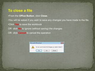
To close a file
•From the Office Button, click Close.
•You will be asked if you wish to save any changes you have made to the file.
•Click Yes to save the workbook
OR click No to ignore (without saving) the changes
OR click Cancel to cancel the operation
To change the text color
• Highlight the text that you want to change color.
• From the Home tab, in the Font group, point to
the Font Color icon.
• Click the arrow just to the right of the Font Color icon.
You'll see some colors appear.
• Select a color to change the text color of the cell.
To align data between the left and right sides of a cell
•Select the cell, or cells, you wish to align.
•On the Home tab, in the Alignment group, click the Align Text Left icon to align
data with the left edge of the cell.
•Click on the Center icon to center data in the cell.
•Click on the Align Text Right icon to align data with the right edge of the cell.
To align data between the top and bottom of a cell
•Select the cell, or cells, you wish to align.
•On the Home tab, in the Alignment group, click the Top
Align icon to align data in the top position of the cell.
•Click on the Middle Align icon to centralized data vertically
in the cell.
•Click the Bottom Align icon to align data in the bottom
position of the cell.
To change the orientation of data cells
•Select the cell, or cells, you wish to change.
•On the Home tab, in the Alignment group, click
the Orientation icon. You will see a drop down
menu allowing you to format the cell orientation.
To wrap multiple lines of data in a cell
• Type the text 'The Ultimate Guide to Excel 2007' into the
cell C5 and press Enter. The entry will appear as one long
line that does not 'fit' into the cell.
• Select the cell C5 and then on the Home tab, in
the Alignment group, click the Wrap Text icon. The text will
wrap as follow
To merge several cells
Select the cells that you wish to merge to become one cell.
On the Home tab, in the Alignment group, click
the Merge & Center icon.
To shrink the text into one cell
•Type the data you require into the cell and press Enter.
•Right-click on the selected cells, click Format Cells.
•From the Format Cells dialog box displayed, click on
the Alignment tab.
•Under the Text control section, tick the Shrink to fit check
box and click on OK.
Hide Column or Row
To hide a column, execute the following steps.
• Open the Excel file.
• To hide the Income column, click on the column D header.
• Right click, and then click on Hide
Unhide Column or Row
To unhide a column, execute the following steps.
• Select the hidden column and the columns on either side
of the hidden column
• Right click on the selected columns and then click on
Unhide.
Conditional formatting in Excel enables you to highlight cells with a certain color,
depending on the cell’s value / or conditions/ or criteria.
Click on Home, Conditional Formatting, Highlight Cells Rules, Greater Than...
Enter the value 80 and select any formatting style
Conditional Formatting
 Sorting data is an integral part of data analysis. You
might want to put a list of names in alphabetical
order, compile a list of product inventory levels
from highest to lowest, or order rows by colors or
icons. Sorting data helps you quickly visualize and
understand your data better, organize and find the
data that you want, and ultimately make more
effective decisions.
 You can sort data by text (A to Z or Z to A),
numbers (smallest to largest or largest to smallest),
and dates and times (oldest to newest and newest to
oldest) in one or more columns.
You can sort your data in descending and ascending order. You can sort
on one column and sort on several criteria at once. To sort in ascending
order, click on the Data tab and then click AZ
Sort in Excel
If you want to sort on several criteria at once, execute the following steps.
Click on the Data tab and then click Sort.
Formulas & Functions
A formula is an expression which calculates the value of a
cell. Functions are predefined formulas and are already available in Excel.
For example, cell A3 below contains a formula which adds the value of cell
A2 to the value of cell A1.
For example, cell A3 below contains the SUM function which calculates
the sum of the range with address A1:A2.
Enter a Formula
To enter a formula, execute the following steps.
1. Select the cell that you want to contain the formula.
2. To let Excel know that you want to enter a formula, type
an equal sign (=).
Note: instead of typing A1 and A2, while typing, simply select cell A1 and cell A2.
Edit a Formula
When you select a cell, Excel shows the value or formula of
the cell in the formula bar.
To edit a formula, click the formula bar and change the formula.
Press enter
Operator Precedence
Excel uses a default order in which calculations occur. If a
part of the formula is in parentheses, that part will be
calculated first. It then performs multiplication or division
calculations. Once this is complete, Excel will add and
subtract the remainder of your formula.
Sum Function
To calculate the sum of a range of cells, execute the following
steps.
1. Select the cell where you want to place the sum /Result
2. Click on the Home tab and then click on
3. Press enter.
Count Function
To count the number of cells of a range, execute the
following steps.
1. Select the cell where you want to place the result.
2. Click on Formulas  Insert Function Select Count
Function  Select the range of cells
3.Press enter.
If Function
The IF function checks whether a condition is met, and
returns one value if TRUE and another value if FALSE.
1. Select cell D2, type in, =IF(A2>2,"That's Correct", "Not
Correct")
The IF function returns one value if a condition you
specify evaluates to TRUE, and another value if that
condition evaluates to FALSE.
For example, the formula =IF(A1>10,"Over 10","10 or
less") returns "Over 10" if A1 is greater than 10, and "10
or less" if A1 is less than or equal to 10.
Syntax
IF(logical_test, value_if_true, [value_if_false])
The IF function syntax has the following arguments :
logical_test . Any value or expression that can be evaluated
to TRUE or FALSE. For example, A10=100 is a logical
expression; if the value in cell A10 is equal to 100, the
expression evaluates to TRUE. Otherwise, the expression
evaluates to FALSE. This argument can use any comparison
calculation operator.
value_if_true The value that you want to be returned if the
logical_test argument evaluates to TRUE. For example, if
the value of this argument is the text string "Within
budget" and the logical_test argument evaluates to TRUE,
the IF function returns the text "Within budget."
value_if_false The value that you want to be returned if the
logical_test argument evaluates to FALSE. For example, if
the value of this argument is the text string "Over budget"
and the logical_test argument evaluates to FALSE, the IF
function returns the text "Over budget."
Cell References in Excel
In Excel and other spreadsheets, reference identifies the location a cell or
group of cells.
Cell references are used in formulas, functions, charts , and other Excel
commands.
Cell references in Excel are very important.
Relative Reference
By default, a spreadsheet cell reference is relative. What this means is that
as a formula or function is copied and pasted to other cells, the cell
references in the formula or function change to reflect the function's new
location.
The reference in the formula is relative to the position of the cell containing
the formula. In other words: each cell references its two neighbors on the left.
Absolute Reference
An absolute cell reference does not change when it a formula is copied
and pasted to other cells.
Absolute cell referencing involves nothing more than placing a dollar
symbol ( $ ) before each letter and number.
 The COUNTIF function counts the number of cells
within a range that meet a single criterion that you
specify. For example, you can count all the cells that
start with a certain letter, or you can count all the cells
that contain a number that is larger or smaller than a
number you specify. For example, suppose you have a
worksheet that contains a list of tasks in column A,
and the first name of the person assigned to each task
in column B. You can use the COUNTIF function to
count how many times a person's name appears in
column B and, in that way, determine how many tasks
are assigned to that person.
For example:
=COUNTIF(B2:B25,"Nancy")
Syntax
COUNTIF(range, criteria)
The COUNTIF function syntax has the following
arguments
Range: One or more cells to count, including numbers or
names, arrays, or references that contain numbers.
Criteria: A number, expression, cell reference, or text
string that defines which cells will be counted. For
example, criteria can be expressed as 32, ">32", B4,
"apples", or "32".
Excel Charts
A chart is a visual representation of data,
in which the data are represented by
symbols such as bars in a bar chart or
lines in a line chart. A chart can represent
tabular numeric data, functions or some
kinds of qualitative structures.
Excel allows to create charts in a variety
of types: Bar Charts, Column Charts, Line
Charts, Area Charts, Scatter Charts, Pie
Charts, Stock Charts.
Excel Charts
A simple chart can say more than a sheet full of numbers. As you'll see,
creating Excel charts is very easy. Here we discuss how to create a chart,
how to switch rows to columns, how to add a chart title, how to change the
legend position, how to change to a different type of chart, and how to
create a pie chart.
To create a chart, open the Excel file.
1. Select the data range you want to include in the chart.
Note: include the headers when selecting the data range!
2. Click on Insert, choose Column under the Charts group, and select one
of the subtypes.
Switch Row/Column
If you want the quarters, displayed on the horizontal
(category) axis, to be displayed on the vertical (value) axis
instead, you can switch rows to columns.
1. Select the chart. The Chart Tools contextual tab activates.
2. Click on the Design tab and click on Switch Row/Column
under the Data group.
Add Chart Title
Our Chart needs a title because at the moment it is unclear
what the numbers represent.
1. Select the chart. The Chart Tools contextual tab activates.
2. On the Layout tab, click on Chart Title, and select Above
Chart.
Change Legend Position
By default, the legend
appears to the right of the
chart. To move the legend to
the bottom of the chart:
1. Select the chart. The
Chart Tools contextual tab
activates.
2. On the Layout tab, click
on Legend and select Show
Legend at Bottom.
Change Chart Type
You can easily change to a different type of chart at any
time.
1. Select the chart. The Chart Tools contextual tab activates.
2. On the Design tab, click on Change Chart Type under the
Type group.
Pie Chart
Pie charts are very useful when you want to display the
contribution of each value (slice) to a total (pie). Use pie
charts when you have only one data series.
1. Select the data range.
2. Click on Insert, choose Pie
under the Charts group,
and select one of the subtypes.
 Using AutoFilter to filter data is a quick and easy way to
find and work with a subset of data in a range of cells or
table. Once you have filtered data in a range of cells or
table, you can either reapply a filter to get up-to-date
results, or clear a filter to redisplay all of the data.
 Filtered data displays only the rows that meet criteria that
you specify and hides rows that you do not want displayed.
After you filter data, you can copy, find, edit, format, chart,
and print the subset of filtered data without rearranging or
moving it.
 You can also filter by more than one column. Filters are
additive, which means that each additional filter is based on
the current filter and further reduces the subset of data
Filter in Excel
You can filter your data If you only want to display records that meet
certain criteria. Click any single cell inside the data set.
Click on the Data tab and then click Filter.
Arrows in the column headers appear.
Now for example, click on the arrow next to Country.
Click on Select All, to clear all the checkboxes.
Next, click the checkbox next to USA.
Click on OK.
To remove the arrows (which will remove the filter as
well), click on Filter from the Data tab again.

More Related Content

What's hot

Introduction to MS excel
Introduction to MS excelIntroduction to MS excel
Introduction to MS excelfatimazaheer12
 
LESSON 3: BASIC SKILLS ON MICROSOFT EXCEL
LESSON 3: BASIC SKILLS ON MICROSOFT EXCELLESSON 3: BASIC SKILLS ON MICROSOFT EXCEL
LESSON 3: BASIC SKILLS ON MICROSOFT EXCELbonzy_30
 
Microsoft Excel- basics
Microsoft Excel-  basicsMicrosoft Excel-  basics
Microsoft Excel- basicsjeshin jose
 
14 must know terms for microsoft excel beginners
14 must know terms for microsoft excel beginners14 must know terms for microsoft excel beginners
14 must know terms for microsoft excel beginnersComputerTutorialsOnline.com
 
ITT PROJECT IN EXCEL AND WORD
ITT PROJECT IN EXCEL AND WORDITT PROJECT IN EXCEL AND WORD
ITT PROJECT IN EXCEL AND WORDAVIRAL161
 
MS Excel Ch 1 PPT
MS Excel Ch 1 PPTMS Excel Ch 1 PPT
MS Excel Ch 1 PPTprsmith72
 
Learn Basic Excel options within 15 minutes
Learn Basic Excel options within 15 minutesLearn Basic Excel options within 15 minutes
Learn Basic Excel options within 15 minutesMohammad rasoolbaig
 
Uses of Excel
Uses of ExcelUses of Excel
Uses of Exceljarleewil
 
Microsoft Office Excel
Microsoft Office ExcelMicrosoft Office Excel
Microsoft Office ExcelvirtualMaryam
 
Introduction to Excel
Introduction to ExcelIntroduction to Excel
Introduction to ExcelNajma Alam
 
Element of an electronic speadsheet ms excel
Element of an electronic speadsheet   ms excelElement of an electronic speadsheet   ms excel
Element of an electronic speadsheet ms exceleVidhya
 
Excel slide show
Excel slide showExcel slide show
Excel slide showRemon sai
 

What's hot (20)

Jayansh computer
Jayansh computerJayansh computer
Jayansh computer
 
Introduction to MS excel
Introduction to MS excelIntroduction to MS excel
Introduction to MS excel
 
LESSON 3: BASIC SKILLS ON MICROSOFT EXCEL
LESSON 3: BASIC SKILLS ON MICROSOFT EXCELLESSON 3: BASIC SKILLS ON MICROSOFT EXCEL
LESSON 3: BASIC SKILLS ON MICROSOFT EXCEL
 
MS Excel 2010 tutorial 6
MS Excel 2010 tutorial 6MS Excel 2010 tutorial 6
MS Excel 2010 tutorial 6
 
Microsoft Excel- basics
Microsoft Excel-  basicsMicrosoft Excel-  basics
Microsoft Excel- basics
 
Basic excel training
Basic excel trainingBasic excel training
Basic excel training
 
14 must know terms for microsoft excel beginners
14 must know terms for microsoft excel beginners14 must know terms for microsoft excel beginners
14 must know terms for microsoft excel beginners
 
Basic Ms excel
Basic Ms excelBasic Ms excel
Basic Ms excel
 
Microsoft Excel Basics
Microsoft Excel BasicsMicrosoft Excel Basics
Microsoft Excel Basics
 
Presentation
PresentationPresentation
Presentation
 
ITT PROJECT IN EXCEL AND WORD
ITT PROJECT IN EXCEL AND WORDITT PROJECT IN EXCEL AND WORD
ITT PROJECT IN EXCEL AND WORD
 
MS Excel Ch 1 PPT
MS Excel Ch 1 PPTMS Excel Ch 1 PPT
MS Excel Ch 1 PPT
 
Learn Basic Excel options within 15 minutes
Learn Basic Excel options within 15 minutesLearn Basic Excel options within 15 minutes
Learn Basic Excel options within 15 minutes
 
Uses of Excel
Uses of ExcelUses of Excel
Uses of Excel
 
02 Excel entering data
02 Excel entering data02 Excel entering data
02 Excel entering data
 
Microsoft Office Excel
Microsoft Office ExcelMicrosoft Office Excel
Microsoft Office Excel
 
Introduction to Excel
Introduction to ExcelIntroduction to Excel
Introduction to Excel
 
Element of an electronic speadsheet ms excel
Element of an electronic speadsheet   ms excelElement of an electronic speadsheet   ms excel
Element of an electronic speadsheet ms excel
 
Excel slide show
Excel slide showExcel slide show
Excel slide show
 
excell
excellexcell
excell
 

Similar to Excel 2007 for Retail

MS EXCEL lecture .pptx
MS EXCEL lecture .pptxMS EXCEL lecture .pptx
MS EXCEL lecture .pptxcityhigh1
 
Excel training basic
Excel training   basicExcel training   basic
Excel training basicTimesRide
 
Training On Microsoft Excel
Training On Microsoft ExcelTraining On Microsoft Excel
Training On Microsoft ExcelTimesRide
 
Getting started with_microsoft_excel
Getting started with_microsoft_excelGetting started with_microsoft_excel
Getting started with_microsoft_excelDeepak Chavan
 
Getting started with_microsoft_excel
Getting started with_microsoft_excelGetting started with_microsoft_excel
Getting started with_microsoft_excelPratiksha Mhatre
 
I am sharing 'ms excel' with you.pptx
I am sharing 'ms excel' with you.pptxI am sharing 'ms excel' with you.pptx
I am sharing 'ms excel' with you.pptxJuneFrancisBarrioTab
 
Advanced Excel Study Materials | Sourav Sir Academy.pptx
Advanced Excel Study Materials | Sourav Sir Academy.pptxAdvanced Excel Study Materials | Sourav Sir Academy.pptx
Advanced Excel Study Materials | Sourav Sir Academy.pptxSBOfficial2
 
cse111-lecture09-1491556611.pptx
cse111-lecture09-1491556611.pptxcse111-lecture09-1491556611.pptx
cse111-lecture09-1491556611.pptxDavid319172
 
Excel for Dummies
Excel for DummiesExcel for Dummies
Excel for DummieseduCBA
 
Basic computer fundamentals_ Microsoft Excel
Basic computer  fundamentals_ Microsoft ExcelBasic computer  fundamentals_ Microsoft Excel
Basic computer fundamentals_ Microsoft ExcelSaraswati yadav
 
Msexcel module 2007
Msexcel module  2007Msexcel module  2007
Msexcel module 2007dhymes
 
22-excel-basics-15511.ppt
22-excel-basics-15511.ppt22-excel-basics-15511.ppt
22-excel-basics-15511.ppt20ArnavKumar8F
 
Excel basics
Excel basicsExcel basics
Excel basicsLotus Yon
 
ms excel for mba first sem students of dr hs gour university sagar(m.p)
ms excel for mba first sem students of dr hs gour university sagar(m.p)ms excel for mba first sem students of dr hs gour university sagar(m.p)
ms excel for mba first sem students of dr hs gour university sagar(m.p)gaurav jain
 
Teaching Excel
Teaching ExcelTeaching Excel
Teaching Excelsam ran
 

Similar to Excel 2007 for Retail (20)

Ms office excel
Ms office excelMs office excel
Ms office excel
 
NCompass Live: Excel for Librarians
NCompass Live: Excel for LibrariansNCompass Live: Excel for Librarians
NCompass Live: Excel for Librarians
 
MS EXCEL lecture .pptx
MS EXCEL lecture .pptxMS EXCEL lecture .pptx
MS EXCEL lecture .pptx
 
Excel training basic
Excel training   basicExcel training   basic
Excel training basic
 
Training On Microsoft Excel
Training On Microsoft ExcelTraining On Microsoft Excel
Training On Microsoft Excel
 
Getting started with_microsoft_excel
Getting started with_microsoft_excelGetting started with_microsoft_excel
Getting started with_microsoft_excel
 
Getting started with_microsoft_excel
Getting started with_microsoft_excelGetting started with_microsoft_excel
Getting started with_microsoft_excel
 
I am sharing 'ms excel' with you.pptx
I am sharing 'ms excel' with you.pptxI am sharing 'ms excel' with you.pptx
I am sharing 'ms excel' with you.pptx
 
kiromax.ppt
kiromax.pptkiromax.ppt
kiromax.ppt
 
Advanced Excel Study Materials | Sourav Sir Academy.pptx
Advanced Excel Study Materials | Sourav Sir Academy.pptxAdvanced Excel Study Materials | Sourav Sir Academy.pptx
Advanced Excel Study Materials | Sourav Sir Academy.pptx
 
cse111-lecture09-1491556611.pptx
cse111-lecture09-1491556611.pptxcse111-lecture09-1491556611.pptx
cse111-lecture09-1491556611.pptx
 
Excel for Dummies
Excel for DummiesExcel for Dummies
Excel for Dummies
 
Basic computer fundamentals_ Microsoft Excel
Basic computer  fundamentals_ Microsoft ExcelBasic computer  fundamentals_ Microsoft Excel
Basic computer fundamentals_ Microsoft Excel
 
Intro to Microsoft Excel 2007
Intro to Microsoft Excel 2007Intro to Microsoft Excel 2007
Intro to Microsoft Excel 2007
 
Msexcel module 2007
Msexcel module  2007Msexcel module  2007
Msexcel module 2007
 
22-excel-basics-15511.ppt
22-excel-basics-15511.ppt22-excel-basics-15511.ppt
22-excel-basics-15511.ppt
 
Excel basics
Excel basicsExcel basics
Excel basics
 
Excel basics
Excel basicsExcel basics
Excel basics
 
ms excel for mba first sem students of dr hs gour university sagar(m.p)
ms excel for mba first sem students of dr hs gour university sagar(m.p)ms excel for mba first sem students of dr hs gour university sagar(m.p)
ms excel for mba first sem students of dr hs gour university sagar(m.p)
 
Teaching Excel
Teaching ExcelTeaching Excel
Teaching Excel
 

More from Soumit Ghosh

Number systems conversions
Number systems conversionsNumber systems conversions
Number systems conversionsSoumit Ghosh
 
Generation Of Computers
Generation Of ComputersGeneration Of Computers
Generation Of ComputersSoumit Ghosh
 
Basics of Operating System
Basics of Operating SystemBasics of Operating System
Basics of Operating SystemSoumit Ghosh
 

More from Soumit Ghosh (6)

Computer Hardware
Computer HardwareComputer Hardware
Computer Hardware
 
Number systems conversions
Number systems conversionsNumber systems conversions
Number systems conversions
 
Networking
NetworkingNetworking
Networking
 
Ms Word
Ms Word Ms Word
Ms Word
 
Generation Of Computers
Generation Of ComputersGeneration Of Computers
Generation Of Computers
 
Basics of Operating System
Basics of Operating SystemBasics of Operating System
Basics of Operating System
 

Recently uploaded

18-04-UA_REPORT_MEDIALITERAСY_INDEX-DM_23-1-final-eng.pdf
18-04-UA_REPORT_MEDIALITERAСY_INDEX-DM_23-1-final-eng.pdf18-04-UA_REPORT_MEDIALITERAСY_INDEX-DM_23-1-final-eng.pdf
18-04-UA_REPORT_MEDIALITERAСY_INDEX-DM_23-1-final-eng.pdfssuser54595a
 
The basics of sentences session 2pptx copy.pptx
The basics of sentences session 2pptx copy.pptxThe basics of sentences session 2pptx copy.pptx
The basics of sentences session 2pptx copy.pptxheathfieldcps1
 
KSHARA STURA .pptx---KSHARA KARMA THERAPY (CAUSTIC THERAPY)————IMP.OF KSHARA ...
KSHARA STURA .pptx---KSHARA KARMA THERAPY (CAUSTIC THERAPY)————IMP.OF KSHARA ...KSHARA STURA .pptx---KSHARA KARMA THERAPY (CAUSTIC THERAPY)————IMP.OF KSHARA ...
KSHARA STURA .pptx---KSHARA KARMA THERAPY (CAUSTIC THERAPY)————IMP.OF KSHARA ...M56BOOKSTORE PRODUCT/SERVICE
 
MENTAL STATUS EXAMINATION format.docx
MENTAL     STATUS EXAMINATION format.docxMENTAL     STATUS EXAMINATION format.docx
MENTAL STATUS EXAMINATION format.docxPoojaSen20
 
Kisan Call Centre - To harness potential of ICT in Agriculture by answer farm...
Kisan Call Centre - To harness potential of ICT in Agriculture by answer farm...Kisan Call Centre - To harness potential of ICT in Agriculture by answer farm...
Kisan Call Centre - To harness potential of ICT in Agriculture by answer farm...Krashi Coaching
 
Employee wellbeing at the workplace.pptx
Employee wellbeing at the workplace.pptxEmployee wellbeing at the workplace.pptx
Employee wellbeing at the workplace.pptxNirmalaLoungPoorunde1
 
Introduction to AI in Higher Education_draft.pptx
Introduction to AI in Higher Education_draft.pptxIntroduction to AI in Higher Education_draft.pptx
Introduction to AI in Higher Education_draft.pptxpboyjonauth
 
ECONOMIC CONTEXT - LONG FORM TV DRAMA - PPT
ECONOMIC CONTEXT - LONG FORM TV DRAMA - PPTECONOMIC CONTEXT - LONG FORM TV DRAMA - PPT
ECONOMIC CONTEXT - LONG FORM TV DRAMA - PPTiammrhaywood
 
CARE OF CHILD IN INCUBATOR..........pptx
CARE OF CHILD IN INCUBATOR..........pptxCARE OF CHILD IN INCUBATOR..........pptx
CARE OF CHILD IN INCUBATOR..........pptxGaneshChakor2
 
Organic Name Reactions for the students and aspirants of Chemistry12th.pptx
Organic Name Reactions  for the students and aspirants of Chemistry12th.pptxOrganic Name Reactions  for the students and aspirants of Chemistry12th.pptx
Organic Name Reactions for the students and aspirants of Chemistry12th.pptxVS Mahajan Coaching Centre
 
Sanyam Choudhary Chemistry practical.pdf
Sanyam Choudhary Chemistry practical.pdfSanyam Choudhary Chemistry practical.pdf
Sanyam Choudhary Chemistry practical.pdfsanyamsingh5019
 
Separation of Lanthanides/ Lanthanides and Actinides
Separation of Lanthanides/ Lanthanides and ActinidesSeparation of Lanthanides/ Lanthanides and Actinides
Separation of Lanthanides/ Lanthanides and ActinidesFatimaKhan178732
 
URLs and Routing in the Odoo 17 Website App
URLs and Routing in the Odoo 17 Website AppURLs and Routing in the Odoo 17 Website App
URLs and Routing in the Odoo 17 Website AppCeline George
 
Enzyme, Pharmaceutical Aids, Miscellaneous Last Part of Chapter no 5th.pdf
Enzyme, Pharmaceutical Aids, Miscellaneous Last Part of Chapter no 5th.pdfEnzyme, Pharmaceutical Aids, Miscellaneous Last Part of Chapter no 5th.pdf
Enzyme, Pharmaceutical Aids, Miscellaneous Last Part of Chapter no 5th.pdfSumit Tiwari
 
How to Make a Pirate ship Primary Education.pptx
How to Make a Pirate ship Primary Education.pptxHow to Make a Pirate ship Primary Education.pptx
How to Make a Pirate ship Primary Education.pptxmanuelaromero2013
 
Solving Puzzles Benefits Everyone (English).pptx
Solving Puzzles Benefits Everyone (English).pptxSolving Puzzles Benefits Everyone (English).pptx
Solving Puzzles Benefits Everyone (English).pptxOH TEIK BIN
 

Recently uploaded (20)

18-04-UA_REPORT_MEDIALITERAСY_INDEX-DM_23-1-final-eng.pdf
18-04-UA_REPORT_MEDIALITERAСY_INDEX-DM_23-1-final-eng.pdf18-04-UA_REPORT_MEDIALITERAСY_INDEX-DM_23-1-final-eng.pdf
18-04-UA_REPORT_MEDIALITERAСY_INDEX-DM_23-1-final-eng.pdf
 
The basics of sentences session 2pptx copy.pptx
The basics of sentences session 2pptx copy.pptxThe basics of sentences session 2pptx copy.pptx
The basics of sentences session 2pptx copy.pptx
 
KSHARA STURA .pptx---KSHARA KARMA THERAPY (CAUSTIC THERAPY)————IMP.OF KSHARA ...
KSHARA STURA .pptx---KSHARA KARMA THERAPY (CAUSTIC THERAPY)————IMP.OF KSHARA ...KSHARA STURA .pptx---KSHARA KARMA THERAPY (CAUSTIC THERAPY)————IMP.OF KSHARA ...
KSHARA STURA .pptx---KSHARA KARMA THERAPY (CAUSTIC THERAPY)————IMP.OF KSHARA ...
 
Model Call Girl in Bikash Puri Delhi reach out to us at 🔝9953056974🔝
Model Call Girl in Bikash Puri  Delhi reach out to us at 🔝9953056974🔝Model Call Girl in Bikash Puri  Delhi reach out to us at 🔝9953056974🔝
Model Call Girl in Bikash Puri Delhi reach out to us at 🔝9953056974🔝
 
MENTAL STATUS EXAMINATION format.docx
MENTAL     STATUS EXAMINATION format.docxMENTAL     STATUS EXAMINATION format.docx
MENTAL STATUS EXAMINATION format.docx
 
Kisan Call Centre - To harness potential of ICT in Agriculture by answer farm...
Kisan Call Centre - To harness potential of ICT in Agriculture by answer farm...Kisan Call Centre - To harness potential of ICT in Agriculture by answer farm...
Kisan Call Centre - To harness potential of ICT in Agriculture by answer farm...
 
Employee wellbeing at the workplace.pptx
Employee wellbeing at the workplace.pptxEmployee wellbeing at the workplace.pptx
Employee wellbeing at the workplace.pptx
 
Introduction to AI in Higher Education_draft.pptx
Introduction to AI in Higher Education_draft.pptxIntroduction to AI in Higher Education_draft.pptx
Introduction to AI in Higher Education_draft.pptx
 
ECONOMIC CONTEXT - LONG FORM TV DRAMA - PPT
ECONOMIC CONTEXT - LONG FORM TV DRAMA - PPTECONOMIC CONTEXT - LONG FORM TV DRAMA - PPT
ECONOMIC CONTEXT - LONG FORM TV DRAMA - PPT
 
CARE OF CHILD IN INCUBATOR..........pptx
CARE OF CHILD IN INCUBATOR..........pptxCARE OF CHILD IN INCUBATOR..........pptx
CARE OF CHILD IN INCUBATOR..........pptx
 
Organic Name Reactions for the students and aspirants of Chemistry12th.pptx
Organic Name Reactions  for the students and aspirants of Chemistry12th.pptxOrganic Name Reactions  for the students and aspirants of Chemistry12th.pptx
Organic Name Reactions for the students and aspirants of Chemistry12th.pptx
 
Sanyam Choudhary Chemistry practical.pdf
Sanyam Choudhary Chemistry practical.pdfSanyam Choudhary Chemistry practical.pdf
Sanyam Choudhary Chemistry practical.pdf
 
Separation of Lanthanides/ Lanthanides and Actinides
Separation of Lanthanides/ Lanthanides and ActinidesSeparation of Lanthanides/ Lanthanides and Actinides
Separation of Lanthanides/ Lanthanides and Actinides
 
Staff of Color (SOC) Retention Efforts DDSD
Staff of Color (SOC) Retention Efforts DDSDStaff of Color (SOC) Retention Efforts DDSD
Staff of Color (SOC) Retention Efforts DDSD
 
URLs and Routing in the Odoo 17 Website App
URLs and Routing in the Odoo 17 Website AppURLs and Routing in the Odoo 17 Website App
URLs and Routing in the Odoo 17 Website App
 
9953330565 Low Rate Call Girls In Rohini Delhi NCR
9953330565 Low Rate Call Girls In Rohini  Delhi NCR9953330565 Low Rate Call Girls In Rohini  Delhi NCR
9953330565 Low Rate Call Girls In Rohini Delhi NCR
 
Enzyme, Pharmaceutical Aids, Miscellaneous Last Part of Chapter no 5th.pdf
Enzyme, Pharmaceutical Aids, Miscellaneous Last Part of Chapter no 5th.pdfEnzyme, Pharmaceutical Aids, Miscellaneous Last Part of Chapter no 5th.pdf
Enzyme, Pharmaceutical Aids, Miscellaneous Last Part of Chapter no 5th.pdf
 
Código Creativo y Arte de Software | Unidad 1
Código Creativo y Arte de Software | Unidad 1Código Creativo y Arte de Software | Unidad 1
Código Creativo y Arte de Software | Unidad 1
 
How to Make a Pirate ship Primary Education.pptx
How to Make a Pirate ship Primary Education.pptxHow to Make a Pirate ship Primary Education.pptx
How to Make a Pirate ship Primary Education.pptx
 
Solving Puzzles Benefits Everyone (English).pptx
Solving Puzzles Benefits Everyone (English).pptxSolving Puzzles Benefits Everyone (English).pptx
Solving Puzzles Benefits Everyone (English).pptx
 

Excel 2007 for Retail

  • 1.
  • 2. Excel is an application that helps to create intricate and dynamic spreadsheets. We can use this robust application to enter numerical values or data into the rows or columns of a spreadsheet, and to use these numerical entries for calculations, charts, formulas, statistical analysis, etc.
  • 3. The first screen that you will see a new blank worksheet that contains grid of cells. This grid is the most important part of the Excel window. It's where you'll perform all your work, such as entering data, writing formulas, and reviewing the results.
  • 4. Microsoft Excel 2007 Workbook and Worksheet A worksheet is the grid of cells where you can type the data. The grid divides your worksheet into rows and columns. Columns are identified with letters (A, B, C … ), while rows are identified with numbers (1, 2, 3 … ). A cell is identified by column and row. For example, B8 is the address of a cell in column B (the second column), and row 8 (the eighth row).
  • 5. A worksheet in Excel 2007 consists of 16,384 columns and over 1 million rows. The worksheets in turn are grouped together into a workbook. By default each workbook in Excel 2007 contains 3 blank worksheets, which are identified by tabs displaying along the bottom of your screen. By default the first worksheet is called Sheet1, the next is Sheet2 and so on.
  • 6. Excel 2007 screen elements •Office button: When clicked, this button opens the Office menu, from which you can open, save, print, and exit as well as the Excel Options button that enables you to change Excel's default settings. •Quick Access Toolbar: A small toolbar next to the Office button contains shortcuts for some of the most common commands such as Save, Undo, and Redo buttons. •Ribbon: A combination of old versions menu bar and toolbar, arranged into a series of tabs ranging from Home through View. Each tab contains buttons, lists, and commands.
  • 7. •Name box: Displays the address of the current active cell where you work in the worksheet. •Formula bar: Displays the address of the active cell on the left edge, and it also shows you the current cell's contents. •Worksheet area: This area contains all the cells of the current worksheet identified by column headings, using letters along the top, and row headings, using numbers along the left edge with tabs for selecting new worksheets. •Zoom control: Use to zoom the Excel screen in or out by dragging the slider.
  • 8. Sheet tabs: Excel 2007 contains 3 blank worksheet tabs by default. Click on the intended tab will go to the particular worksheet. •Status bar: Reports information about the worksheet and provides shortcuts for changing the view and the zoom.
  • 9. To enter text into a worksheet •Select the cell in which you want to enter the text. •Type in the text/data into the cell. •Press the Enter key. Text entries are left aligned by default. To enter numbers into a worksheet •Select the cell in which you want to enter a number. •Type in the number into the cell and press Enter. •If you want to enter a negative number, type a minus sign in front of it or enclose it in parentheses (bracket), e.g. -15 or (15). •To indicate decimal places, you type a full stop such as 125.89. •The numbers will be right aligned by default.
  • 10. To enter dates and times into a worksheet • Select the cell in which you want to enter the date or time. • Type in the date or time. Separate the date with either hyphens (-) or slashes (/). • Press Enter. • To enter the current date, press Ctrl+; • To enter the current time, press Ctrl+:
  • 11. To save a workbook • From Office Button, click Save OR Click the Save button on the Quick Access Toolbar. • From the Save As dialog box displayed, ensure that you browse to the folder/disk drive that you would like to save the file. • Enter the file name in the File name: text box. The file name can be up to 255 characters in length. • Click on the Save button.
  • 12. To save a backup copy (subsequent times) •From the Office Button, point to Save As and click Excel Workbook. •Enter a name in the File name: text box. •Click on the Save button. Note: By default, Excel saves a copy of your work automatically every ten minutes. To adjust this setting (or turn if off), use the Save tab of the Excel Options dialog box (Office Button - Excel Options).
  • 13. To close a file •From the Office Button, click Close. •You will be asked if you wish to save any changes you have made to the file. •Click Yes to save the workbook OR click No to ignore (without saving) the changes OR click Cancel to cancel the operation
  • 14. To change the text color • Highlight the text that you want to change color. • From the Home tab, in the Font group, point to the Font Color icon. • Click the arrow just to the right of the Font Color icon. You'll see some colors appear. • Select a color to change the text color of the cell.
  • 15. To align data between the left and right sides of a cell •Select the cell, or cells, you wish to align. •On the Home tab, in the Alignment group, click the Align Text Left icon to align data with the left edge of the cell. •Click on the Center icon to center data in the cell. •Click on the Align Text Right icon to align data with the right edge of the cell.
  • 16. To align data between the top and bottom of a cell •Select the cell, or cells, you wish to align. •On the Home tab, in the Alignment group, click the Top Align icon to align data in the top position of the cell. •Click on the Middle Align icon to centralized data vertically in the cell. •Click the Bottom Align icon to align data in the bottom position of the cell.
  • 17. To change the orientation of data cells •Select the cell, or cells, you wish to change. •On the Home tab, in the Alignment group, click the Orientation icon. You will see a drop down menu allowing you to format the cell orientation.
  • 18. To wrap multiple lines of data in a cell • Type the text 'The Ultimate Guide to Excel 2007' into the cell C5 and press Enter. The entry will appear as one long line that does not 'fit' into the cell. • Select the cell C5 and then on the Home tab, in the Alignment group, click the Wrap Text icon. The text will wrap as follow
  • 19. To merge several cells Select the cells that you wish to merge to become one cell. On the Home tab, in the Alignment group, click the Merge & Center icon.
  • 20. To shrink the text into one cell •Type the data you require into the cell and press Enter. •Right-click on the selected cells, click Format Cells. •From the Format Cells dialog box displayed, click on the Alignment tab. •Under the Text control section, tick the Shrink to fit check box and click on OK.
  • 21. Hide Column or Row To hide a column, execute the following steps. • Open the Excel file. • To hide the Income column, click on the column D header. • Right click, and then click on Hide
  • 22. Unhide Column or Row To unhide a column, execute the following steps. • Select the hidden column and the columns on either side of the hidden column • Right click on the selected columns and then click on Unhide.
  • 23. Conditional formatting in Excel enables you to highlight cells with a certain color, depending on the cell’s value / or conditions/ or criteria. Click on Home, Conditional Formatting, Highlight Cells Rules, Greater Than... Enter the value 80 and select any formatting style Conditional Formatting
  • 24.  Sorting data is an integral part of data analysis. You might want to put a list of names in alphabetical order, compile a list of product inventory levels from highest to lowest, or order rows by colors or icons. Sorting data helps you quickly visualize and understand your data better, organize and find the data that you want, and ultimately make more effective decisions.  You can sort data by text (A to Z or Z to A), numbers (smallest to largest or largest to smallest), and dates and times (oldest to newest and newest to oldest) in one or more columns.
  • 25. You can sort your data in descending and ascending order. You can sort on one column and sort on several criteria at once. To sort in ascending order, click on the Data tab and then click AZ Sort in Excel If you want to sort on several criteria at once, execute the following steps. Click on the Data tab and then click Sort.
  • 26. Formulas & Functions A formula is an expression which calculates the value of a cell. Functions are predefined formulas and are already available in Excel. For example, cell A3 below contains a formula which adds the value of cell A2 to the value of cell A1. For example, cell A3 below contains the SUM function which calculates the sum of the range with address A1:A2.
  • 27. Enter a Formula To enter a formula, execute the following steps. 1. Select the cell that you want to contain the formula. 2. To let Excel know that you want to enter a formula, type an equal sign (=). Note: instead of typing A1 and A2, while typing, simply select cell A1 and cell A2.
  • 28. Edit a Formula When you select a cell, Excel shows the value or formula of the cell in the formula bar. To edit a formula, click the formula bar and change the formula. Press enter
  • 29. Operator Precedence Excel uses a default order in which calculations occur. If a part of the formula is in parentheses, that part will be calculated first. It then performs multiplication or division calculations. Once this is complete, Excel will add and subtract the remainder of your formula.
  • 30. Sum Function To calculate the sum of a range of cells, execute the following steps. 1. Select the cell where you want to place the sum /Result 2. Click on the Home tab and then click on 2. Click on the Home tab and then click on 3. Press enter.
  • 31. Count Function To count the number of cells of a range, execute the following steps. 1. Select the cell where you want to place the result. 2. Click on Formulas  Insert Function Select Count Function  Select the range of cells 3.Press enter.
  • 32. If Function The IF function checks whether a condition is met, and returns one value if TRUE and another value if FALSE. 1. Select cell D2, type in, =IF(A2>2,"That's Correct", "Not Correct")
  • 33. The IF function returns one value if a condition you specify evaluates to TRUE, and another value if that condition evaluates to FALSE. For example, the formula =IF(A1>10,"Over 10","10 or less") returns "Over 10" if A1 is greater than 10, and "10 or less" if A1 is less than or equal to 10. Syntax IF(logical_test, value_if_true, [value_if_false])
  • 34. The IF function syntax has the following arguments : logical_test . Any value or expression that can be evaluated to TRUE or FALSE. For example, A10=100 is a logical expression; if the value in cell A10 is equal to 100, the expression evaluates to TRUE. Otherwise, the expression evaluates to FALSE. This argument can use any comparison calculation operator. value_if_true The value that you want to be returned if the logical_test argument evaluates to TRUE. For example, if the value of this argument is the text string "Within budget" and the logical_test argument evaluates to TRUE, the IF function returns the text "Within budget." value_if_false The value that you want to be returned if the logical_test argument evaluates to FALSE. For example, if the value of this argument is the text string "Over budget" and the logical_test argument evaluates to FALSE, the IF function returns the text "Over budget."
  • 35. Cell References in Excel In Excel and other spreadsheets, reference identifies the location a cell or group of cells. Cell references are used in formulas, functions, charts , and other Excel commands. Cell references in Excel are very important. Relative Reference By default, a spreadsheet cell reference is relative. What this means is that as a formula or function is copied and pasted to other cells, the cell references in the formula or function change to reflect the function's new location. The reference in the formula is relative to the position of the cell containing the formula. In other words: each cell references its two neighbors on the left.
  • 36. Absolute Reference An absolute cell reference does not change when it a formula is copied and pasted to other cells. Absolute cell referencing involves nothing more than placing a dollar symbol ( $ ) before each letter and number.
  • 37.  The COUNTIF function counts the number of cells within a range that meet a single criterion that you specify. For example, you can count all the cells that start with a certain letter, or you can count all the cells that contain a number that is larger or smaller than a number you specify. For example, suppose you have a worksheet that contains a list of tasks in column A, and the first name of the person assigned to each task in column B. You can use the COUNTIF function to count how many times a person's name appears in column B and, in that way, determine how many tasks are assigned to that person.
  • 38. For example: =COUNTIF(B2:B25,"Nancy") Syntax COUNTIF(range, criteria) The COUNTIF function syntax has the following arguments Range: One or more cells to count, including numbers or names, arrays, or references that contain numbers. Criteria: A number, expression, cell reference, or text string that defines which cells will be counted. For example, criteria can be expressed as 32, ">32", B4, "apples", or "32".
  • 39. Excel Charts A chart is a visual representation of data, in which the data are represented by symbols such as bars in a bar chart or lines in a line chart. A chart can represent tabular numeric data, functions or some kinds of qualitative structures. Excel allows to create charts in a variety of types: Bar Charts, Column Charts, Line Charts, Area Charts, Scatter Charts, Pie Charts, Stock Charts.
  • 40. Excel Charts A simple chart can say more than a sheet full of numbers. As you'll see, creating Excel charts is very easy. Here we discuss how to create a chart, how to switch rows to columns, how to add a chart title, how to change the legend position, how to change to a different type of chart, and how to create a pie chart. To create a chart, open the Excel file. 1. Select the data range you want to include in the chart. Note: include the headers when selecting the data range! 2. Click on Insert, choose Column under the Charts group, and select one of the subtypes.
  • 41. Switch Row/Column If you want the quarters, displayed on the horizontal (category) axis, to be displayed on the vertical (value) axis instead, you can switch rows to columns. 1. Select the chart. The Chart Tools contextual tab activates. 2. Click on the Design tab and click on Switch Row/Column under the Data group.
  • 42. Add Chart Title Our Chart needs a title because at the moment it is unclear what the numbers represent. 1. Select the chart. The Chart Tools contextual tab activates. 2. On the Layout tab, click on Chart Title, and select Above Chart.
  • 43. Change Legend Position By default, the legend appears to the right of the chart. To move the legend to the bottom of the chart: 1. Select the chart. The Chart Tools contextual tab activates. 2. On the Layout tab, click on Legend and select Show Legend at Bottom.
  • 44. Change Chart Type You can easily change to a different type of chart at any time. 1. Select the chart. The Chart Tools contextual tab activates. 2. On the Design tab, click on Change Chart Type under the Type group.
  • 45. Pie Chart Pie charts are very useful when you want to display the contribution of each value (slice) to a total (pie). Use pie charts when you have only one data series. 1. Select the data range. 2. Click on Insert, choose Pie under the Charts group, and select one of the subtypes.
  • 46.  Using AutoFilter to filter data is a quick and easy way to find and work with a subset of data in a range of cells or table. Once you have filtered data in a range of cells or table, you can either reapply a filter to get up-to-date results, or clear a filter to redisplay all of the data.  Filtered data displays only the rows that meet criteria that you specify and hides rows that you do not want displayed. After you filter data, you can copy, find, edit, format, chart, and print the subset of filtered data without rearranging or moving it.  You can also filter by more than one column. Filters are additive, which means that each additional filter is based on the current filter and further reduces the subset of data
  • 47. Filter in Excel You can filter your data If you only want to display records that meet certain criteria. Click any single cell inside the data set. Click on the Data tab and then click Filter. Arrows in the column headers appear. Now for example, click on the arrow next to Country. Click on Select All, to clear all the checkboxes. Next, click the checkbox next to USA. Click on OK. To remove the arrows (which will remove the filter as well), click on Filter from the Data tab again.