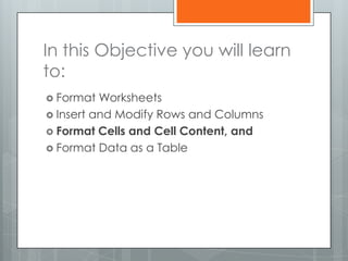
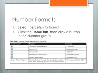
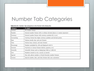
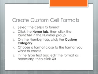
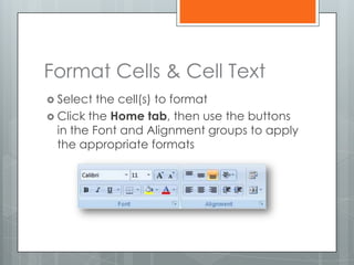
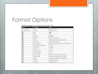
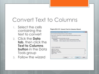
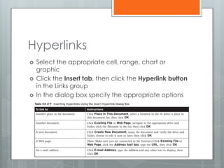
This document provides instructions for formatting worksheets in Microsoft Excel 2007. It covers topics such as formatting cells and cell content through number formats, styles, fonts, borders, and fill colors. Additional topics include inserting and modifying rows and columns, converting text to columns, splitting and merging cells, and adding hyperlinks. The objective is to teach the user how to properly format data and content within Excel worksheets.

1. Microsoft
Excel 2007
Objective 2: Formatting
Data and Content

2. In this Objective you will learn
to:
 Format Worksheets
 Insert and Modify Rows and Columns
 Format Cells and Cell Content, and
 Format Data as a Table

3. Formatting Cells & Cell
Content
• Using Number Formats • Format Text
• Creating Custom Cell • Convert text to columns,
Formats • Split and Merge
• Apply Quick Styles • Cell Borders and Fill Colors
• Create and Apply a • Hyperlinks
Custom Style

4. Number Formats
1. Select the cell(s) to format
2. Click the Home tab, then click a button
in the Number group

5. Number Tab Categories

6. Create Custom Cell Formats
1. Select the cell(s) to format
2. Click the Home tab, then click the
launcher in the Number group
3. On the Number tab, click the Custom
category
4. Choose a format close to the format you
want to create
5. In the Type text box, edit the format as
necessary, then click OK

7. Apply Cell Quick Styles
 Select the cell(s) to
format
 Click the Home
tab, then click the
Cell Styles button in
the Styles group,
then click a style in
one of the groups

8. Create and Apply a Custom
Style
 Select the cell(s) to
format
 Click the Home
tab, then click the
Cell Styles button in
the Styles
group, then click
New Cell Style
 Follow the
instructions that
appear

9. Format Cells & Cell Text
 Select the cell(s) to format
 Click the Home tab, then use the buttons
in the Font and Alignment groups to apply
the appropriate formats

10. Format Options

11. Convert Text to Columns
1. Select the cells
containing the
text to convert
2. Click the Data
tab, then click the
Text to Columns
button in the Data
Tools group
3. Follow the wizard

12. Split and Merge Cells
1. Select the cells to merge or the merged
cell to be split
2. Click the Home tab, then click the Merge
and Center list arrow in the Alignment
group
3. Choose the appropriate option

13. Format Cell Borders and Fill
Colors
1. Select the cell(s) to format
Cell Borders
 Click the Home tab, then click the Borders
list arrow in the Font group, then click an
appropriate border option
Fill Color
 Click the Home tab, then click the Fill
Color list arrow in the Font group, then
click an appropriate color

14. Hyperlinks
 Select the appropriate cell, range, chart or
graphic
 Click the Insert tab, then click the Hyperlink button
in the Links group
 In the dialog box specify the appropriate options

15. Lesson Review Activity
1. Open a new workbook
2. Type 100 in cell A1, B1, and C1
3. Practice using the different number formats
by setting A1 to currency, B1 to
Percentage, and C1 to Accounting
4. Select the Accent 1 cell style for A1, the
Accent 4 style for B1 and the Accent 5 style
for C1
5. Create your own Cell style and apply it to
cell C1

16. Lesson Review Activity
6. Type your name in cell A2 and change that
text into 2 columns
7. In cell A3 type Office Computer Applications
8. Merge and Center that text from A1:C1
9. Apply an outside border to the new merged
cell and fill it with a green color
10. In cell A4 type Google, then create a
hyperlink to www.google.com
11. Save as Cell Formats when complete