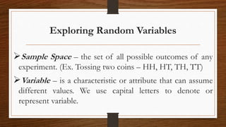
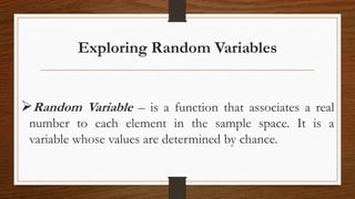
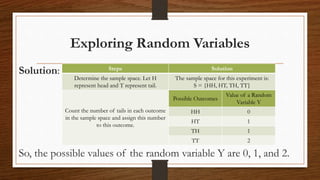
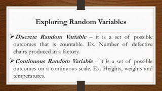
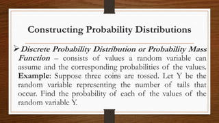
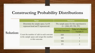
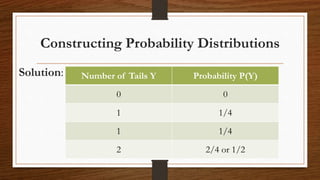
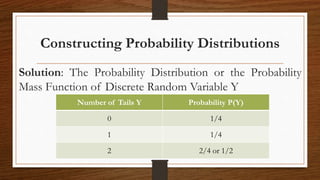
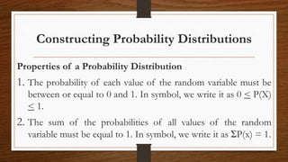
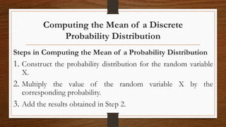
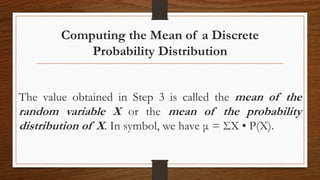
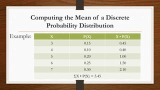
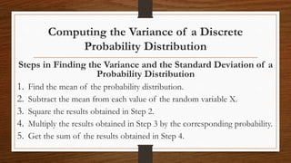
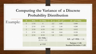
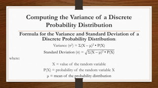
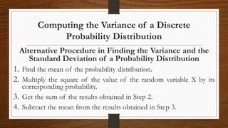
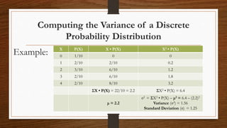
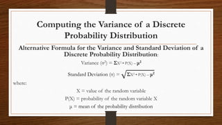
This document introduces key concepts related to random variables and probability distributions: - A random variable is a function that assigns a numerical value to each possible outcome of an experiment. Random variables can be discrete or continuous. - A probability distribution specifies the possible values of a random variable and their probabilities. For discrete random variables, this is called a probability mass function. - Key properties of a probability distribution are that each probability is between 0 and 1, and the sum of all probabilities equals 1. - The mean, variance, and standard deviation can be calculated from a probability distribution. The mean is the expected value, while variance and standard deviation measure dispersion around the mean.

1. Chapter 1
Random Variables and Probability
Distributions
Mr. Anthony F. Balatar Jr.
Subject Instructor

2. Exploring Random Variables
Sample Space – the set of all possible outcomes of any
experiment. (Ex. Tossing two coins – HH, HT, TH, TT)
Variable – is a characteristic or attribute that can assume
different values. We use capital letters to denote or
represent variable.

3. Exploring Random Variables
Random Variable – is a function that associates a real
number to each element in the sample space. It is a
variable whose values are determined by chance.

4. Exploring Random Variables
Example: Suppose three coins are tossed. Let Y be the
random variable representing the number of tails. Find the
values of the random variable Y. Complete the table below.
Possible Outcomes Value of a Random Variable Y
HH
HT
TH
TT

5. Exploring Random Variables
Solution:
So, the possible values of the random variable Y are 0, 1, and 2.
Steps Solution
Determine the sample space. Let H
represent head and T represent tail.
The sample space for this experiment is:
S = {HH, HT, TH, TT}
Count the number of tails in each outcome
in the sample space and assign this number
to this outcome.
Possible Outcomes
Value of a Random
Variable Y
HH 0
HT 1
TH 1
TT 2

6. Exploring Random Variables
Discrete Random Variable – it is a set of possible
outcomes that is countable. Ex. Number of defective
chairs produced in a factory.
Continuous Random Variable – it is a set of possible
outcomes on a continuous scale. Ex. Heights, weights and
temperatures.

7. Constructing Probability Distributions
Discrete Probability Distribution or Probability Mass
Function – consists of values a random variable can
assume and the corresponding probabilities of the values.
Example: Suppose three coins are tossed. Let Y be the
random variable representing the number of tails that
occur. Find the probability of each of the values of the
random variable Y.

8. Constructing Probability Distributions
Solution:

9. Constructing Probability Distributions
Solution: Number of Tails Y Probability P(Y)
0 0
1 1/4
1 1/4
2 2/4 or 1/2

10. Constructing Probability Distributions
Solution: The Probability Distribution or the Probability
Mass Function of Discrete Random Variable Y
Number of Tails Y Probability P(Y)
0 1/4
1 1/4
2 2/4 or 1/2

11. Constructing Probability Distributions
Properties of a Probability Distribution
1. The probability of each value of the random variable must be
between or equal to 0 and 1. In symbol, we write it as 0 < P(X)
< 1.
2. The sum of the probabilities of all values of the random
variable must be equal to 1. In symbol, we write it as ΣP(x) = 1.

12. Computing the Mean of a Discrete
Probability Distribution
Steps in Computing the Mean of a Probability Distribution
1. Construct the probability distribution for the random variable
X.
2. Multiply the value of the random variable X by the
corresponding probability.
3. Add the results obtained in Step 2.

13. Computing the Mean of a Discrete
Probability Distribution
The value obtained in Step 3 is called the mean of the
random variable X or the mean of the probability
distribution of X. In symbol, we have μ = ΣX • P(X).

14. Computing the Mean of a Discrete
Probability Distribution
Example: X P(X) X • P(X)
3 0.15 0.45
4 0.10 0.40
5 0.20 1.00
6 0.25 1.50
7 0.30 2.10
ΣX • P(X) = 5.45

15. Computing the Variance of a Discrete
Probability Distribution
Steps in Finding the Variance and the Standard Deviation of a
Probability Distribution
1. Find the mean of the probability distribution.
2. Subtract the mean from each value of the random variable X.
3. Square the results obtained in Step 2.
4. Multiply the results obtained in Step 3 by the corresponding probability.
5. Get the sum of the results obtained in Step 4.

16. Computing the Variance of a Discrete
Probability Distribution
Example: X P(X) X • P(X) X - μ (X – μ)2 (X – μ)2 • P(X)
0 1/10 0 -2.2 4.84 0.484
1 2/10 2/10 -1.2 1.44 0.288
2 3/10 6/10 -0.2 0.04 0.012
3 2/10 6/10 0.8 0.64 0.128
4 2/10 8/10 1.8 3.24 0.648
ΣX • P(X) =
22/10 = 2.2
Σ(X – μ)2 • P(X) = 1.56
μ = 2.2
Variance = 1.56
Standard Deviation = 1.25

17. Computing the Variance of a Discrete
Probability Distribution
Formula for the Variance and Standard Deviation of a
Discrete Probability Distribution:
Variance (σ2) = Σ(X – μ)2 • P(X)
Standard Deviation (σ) = Σ(X – μ)2 • P(X)
where:
X = value of the random variable
P(X) = probability of the random variable X
μ = mean of the probability distribution

18. Computing the Variance of a Discrete
Probability Distribution
Alternative Procedure in Finding the Variance and the
Standard Deviation of a Probability Distribution
1. Find the mean of the probability distribution.
2. Multiply the square of the value of the random variable X by its
corresponding probability.
3. Get the sum of the results obtained in Step 2.
4. Subtract the mean from the results obtained in Step 3.

19. Computing the Variance of a Discrete
Probability Distribution
Example: X P(X) X • P(X) X2 • P(X)
0 1/10 0 0
1 2/10 2/10 0.2
2 3/10 6/10 1.2
3 2/10 6/10 1.8
4 2/10 8/10 3.2
ΣX • P(X) = 22/10 = 2.2 ΣX2 • P(X) = 6.4
μ = 2.2
σ2 = ΣX2 • P(X) – μ2 = 6.4 – (2.2)2
Variance (σ2) = 1.56
Standard Deviation (σ) = 1.25

20. Computing the Variance of a Discrete
Probability Distribution
Alternative Formula for the Variance and Standard Deviation of a
Discrete Probability Distribution:
Variance (σ2) = ΣX2 • P(X) – μ2
Standard Deviation (σ) = ΣX2 • P(X) – μ2
where:
X = value of the random variable
P(X) = probability of the random variable X
μ = mean of the probability distribution