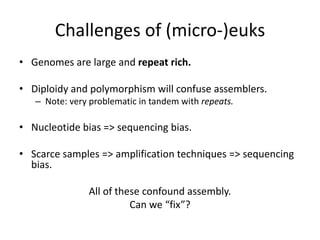
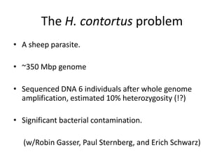
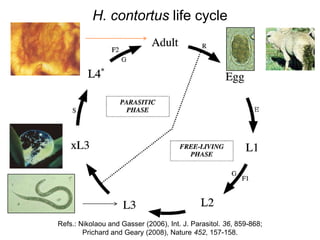
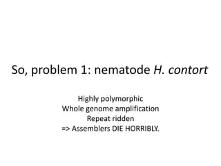
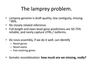
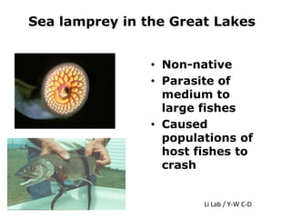
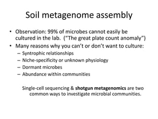
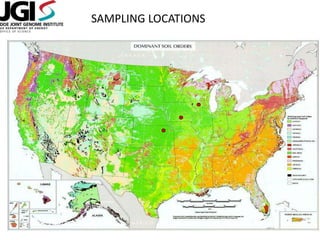
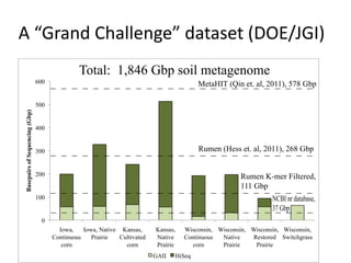
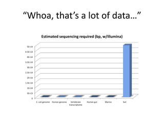
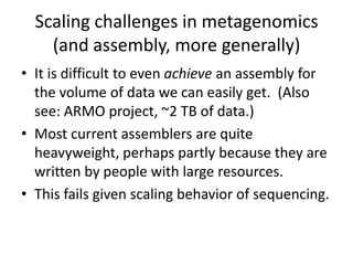
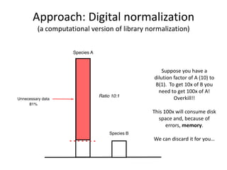
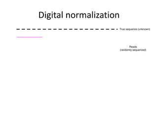
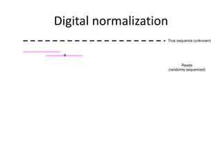
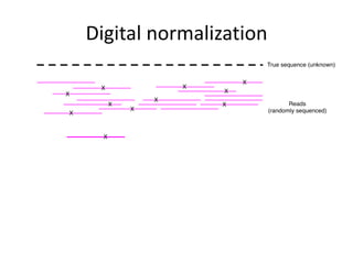
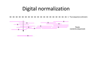
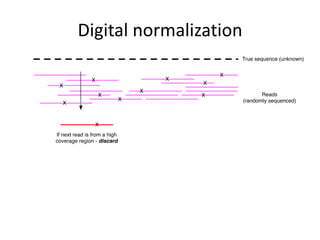
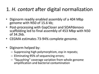
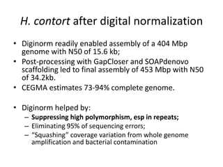
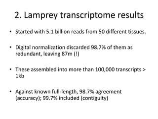
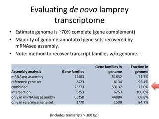
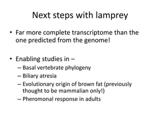
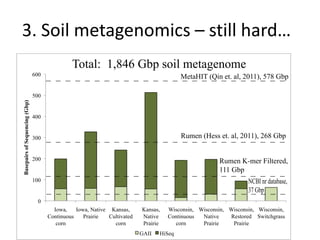
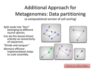
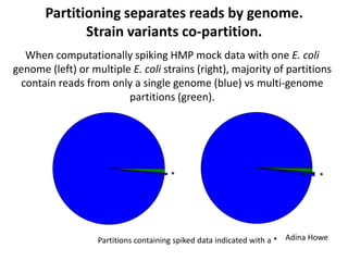
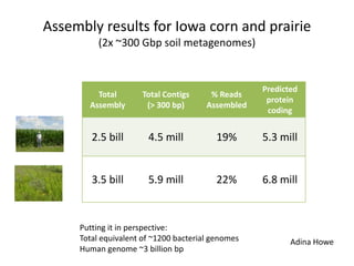
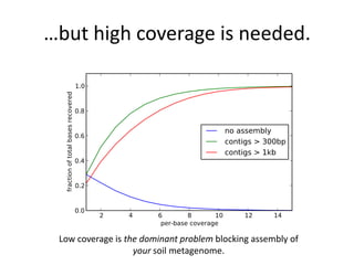
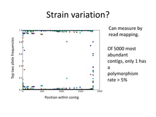
C. Titus Brown
Assistant Professor
CSE, MMG, BEACON
Michigan State University
ctb@msu.edu
The pro-shotgun-assembly talk.
Acknowledgements
Lab members involved Collaborators
• Adina Howe (w/Tiedje)
• Jason Pell
• Arend Hintze
• Rosangela Canino-Koning
• Qingpeng Zhang
• Elijah Lowe
• Likit Preeyanon
• Jiarong Guo
• Tim Brom
• Kanchan Pavangadkar
• Eric McDonald
• Jordan Fish
• Chris Welcher
• Jim Tiedje, MSU
• Billie Swalla, UW
• Janet Jansson, LBNL
• Susannah Tringe, JGI
Funding
USDA NIFA; NSF IOS;
BEACON.
Open, online science
All of the software and approaches I’m talking about
today are available:
Assembling large, complex metagenomes
arxiv.org/abs/1212.2832
khmer software:
github.com/ged-lab/khmer/
Blog: http://ivory.idyll.org/blog/
Twitter: @ctitusbrown
Note: I am phylogenetically
unconstrained…
• Chordate mRNAseq (Molgula + lamprey +
chick)
• Nematode genomics
• Soil metagenomics
…but so far not microbial euks, specifically.
My goals in this work
• Interested in genes & genomes: function &
evolution, but not as much taxonomy.
• Little or no marker work (16s/18s)
• Develop lightweight prefiltering techniques for
other tools.
• Software & methods => democritize data
analysis.
I am unambiguously pro-assembly.
• Short-read analysis can be misleading; need more work like Doc
Pollard’s showing where/why!
• Assembly reduces the data size, increases boinformatic signal,
and eliminates random errors.
• The general mental frameworks (OLC or DBG) underpin virtually
all sequence analysis anyway, note.
• So, why not?
– Assembly is HARD, SLOW, TRICKY.
– Assemblies may MISLEAD you.
– Assembly is a STRINGENT FILTER on your data <=> heuristics.
There is quite a bit of life left to sequence & assemble.
http://pacelab.colorado.edu/
Challenges of (micro-)euks
• Genomes are large and repeat rich.
• Diploidy and polymorphism will confuse assemblers.
– Note: very problematic in tandem with repeats.
• Nucleotide bias => sequencing bias.
• Scarce samples => amplification techniques => sequencing
bias.
All of these confound assembly.
Can we “fix”?
Three illustrative problem cases
• H. contortus genome assembly.
• Lamprey reference-free transcriptome
assembly.
• Soil metagenome assembly.
The H. contortus problem
• A sheep parasite.
• ~350 Mbp genome
• Sequenced DNA 6 individuals after whole genome
amplification, estimated 10% heterozygosity (!?)
• Significant bacterial contamination.
(w/Robin Gasser, Paul Sternberg, and Erich Schwarz)
H. contortus life cycle
Refs.: Nikolaou and Gasser (2006), Int. J. Parasitol. 36, 859-868;
Prichard and Geary (2008), Nature 452, 157-158.
The power of next-gen. sequencing:
get 180x coverage ... and then watch your
assemblies never finish
Libraries built and sequenced:
300-nt inserts, 2x75 nt paired-end reads
500-nt inserts, 2x75 and 2x100 nt paired-end reads
2-kb, 5-kb, and 10-kb inserts, 2x49 nt paired-end reads
Nothing would assemble at all until filtered for basic quality.
Filtering let ≤500 nt-sized inserts to assemble in a mere week.
But 2+ kb-sized inserts would not assemble even then.
Erich Schwarz
So, problem 1: nematode H. contort
Highly polymorphic
Whole genome amplification
Repeat ridden
=> Assemblers DIE HORRIBLY.
The lamprey problem.
• Lamprey genome is draft quality; low contiguity, missing
~30%.
• No closely related reference.
• Full-length and exon-level gene predictions are 50-75%
reliable, and rarely capture UTRs / isoforms.
• De novo assembly, if we do it well, can identify
– Novel genes
– Novel exons
– Fast evolving genes
• Somatic recombination: how much are we missing, really?
Sea lamprey in the Great Lakes
• Non-native
• Parasite of
medium to
large fishes
• Caused
populations of
host fishes to
crash
Li Lab / Y-W C-D
Lamprey transcrpitome
• Started with 5.1 billion reads from 50 different
tissues.
No assembler on the planet can handle this
much data.
So, problem 2: lamprey mRNAseq
Must go with reference-free approach.
TOO MUCH DATA.
Soil metagenome assembly
• Observation: 99% of microbes cannot easily be
cultured in the lab. (“The great plate count anomaly”)
• Many reasons why you can’t or don’t want to culture:
– Syntrophic relationships
– Niche-specificity or unknown physiology
– Dormant microbes
– Abundance within communities
Single-cell sequencing & shotgun metagenomics are two
common ways to investigate microbial communities.
SAMPLING LOCATIONS
Investigating soil microbial ecology
• What ecosystem level functions are present, and
how do microbes do them?
• How does agricultural soil differ from native soil?
• How does soil respond to climate perturbation?
• Questions that are not easy to answer without
shotgun sequencing:
– What kind of strain-level heterogeneity is present in
the population?
– What does the phage and viral population look like?
– What species are where?
A “Grand Challenge” dataset (DOE/JGI)
0
100
200
300
400
500
600
Iowa,
Continuous
corn
Iowa, Native
Prairie
Kansas,
Cultivated
corn
Kansas,
Native
Prairie
Wisconsin,
Continuous
corn
Wisconsin,
Native
Prairie
Wisconsin,
Restored
Prairie
Wisconsin,
Switchgrass
BasepairsofSequencing(Gbp)
GAII HiSeq
Rumen (Hess et. al, 2011), 268 Gbp
MetaHIT (Qin et. al, 2011), 578 Gbp
NCBI nr database,
37 Gbp
Total: 1,846 Gbp soil metagenome
Rumen K-mer Filtered,
111 Gbp
“Whoa, that’s a lot of data…”
0
5E+13
1E+14
1.5E+14
2E+14
2.5E+14
3E+14
3.5E+14
4E+14
4.5E+14
5E+14
E. coli genome Human genome Vertebrate
transcriptome
Human gut Marine Soil
Estimated sequencing required (bp, w/Illumina)
Scaling challenges in metagenomics
(and assembly, more generally)
• It is difficult to even achieve an assembly for
the volume of data we can easily get. (Also
see: ARMO project, ~2 TB of data.)
• Most current assemblers are quite
heavyweight, perhaps partly because they are
written by people with large resources.
• This fails given scaling behavior of sequencing.
So, problem 3: soil metagenomics
TOO MUCH DATA.
BAD SCALING.
Approach: Digital normalization
(a computational version of library normalization)
Suppose you have a
dilution factor of A (10) to
B(1). To get 10x of B you
need to get 100x of A!
Overkill!!
This 100x will consume disk
space and, because of
errors, memory.
We can discard it for you…
Digital normalization
Digital normalization approach
A digital analog to cDNA library normalization, diginorm:
• Reference free.
• Is single pass: looks at each read only once;
• Does not “collect” the majority of errors;
• Keeps all low-coverage reads;
• Smooths out coverage of regions.
Coverage before digital normalization:
(MD amplified)
Coverage after digital normalization:
Normalizes coverage
Discards redundancy
Eliminates majority of
errors
Scales assembly dramatically.
Assembly is 98% identical.
Wait, that works??
Note, digital normalization is freely available, with lots of tutorials.
Derived approach now part of Trinity (Broad mRNAseq assembler).
It is, ahem, still unpublished, but available on arXiv:
arxiv.org/abs/1203.4802
1. H. contort after digital normalization
• Diginorm readily enabled assembly of a 404 Mbp
genome with N50 of 15.6 kb;
• Post-processing with GapCloser and SOAPdenovo
scaffolding led to final assembly of 453 Mbp with N50
of 34.2kb.
• CEGMA estimates 73-94% complete genome.
• Diginorm helped by:
– Suppressing high polymorphism, esp in repeats;
– Eliminating 95% of sequencing errors;
– “Squashing” coverage variation from whole genome
amplification and bacterial contamination
H. contort after digital normalization
• Diginorm readily enabled assembly of a 404 Mbp
genome with N50 of 15.6 kb;
• Post-processing with GapCloser and SOAPdenovo
scaffolding led to final assembly of 453 Mbp with N50
of 34.2kb.
• CEGMA estimates 73-94% complete genome.
• Diginorm helped by:
– Suppressing high polymorphism, esp in repeats;
– Eliminating 95% of sequencing errors;
– “Squashing” coverage variation from whole genome
amplification and bacterial contamination
Next steps with H. contortus
• Publish the genome paper 
• Identification of antibiotic targets for
treatment in agricultural settings (animal
husbandry).
• Serving as “reference approach” for a wide
variety of parasitic nematodes, many of which
have similar genomic issues.
2. Lamprey transcriptome results
• Started with 5.1 billion reads from 50 different tissues.
• Digital normalization discarded 98.7% of them as
redundant, leaving 87m (!)
• These assembled into more than 100,000 transcripts >
1kb
• Against known full-length, 98.7% agreement
(accuracy); 99.7% included (contiguity)
Evaluating de novo lamprey
transcriptome
• Estimate genome is ~70% complete (gene complement)
• Majority of genome-annotated gene sets recovered by
mRNAseq assembly.
• Note: method to recover transcript families w/o genome…
Assembly analysis Gene families
Gene families in
genome
Fraction in
genome
mRNAseq assembly 72003 51632 71.7%
reference gene set 8523 8134 95.4%
combined 73773 53137 72.0%
intersection 6753 6753 100.0%
only in mRNAseq assembly 65250 44884 68.8%
only in reference gene set 1770 1500 84.7%
(Includes transcripts > 300 bp)
Next steps with lamprey
• Far more complete transcriptome than the
one predicted from the genome!
• Enabling studies in –
– Basal vertebrate phylogeny
– Biliary atresia
– Evolutionary origin of brown fat (previously
thought to be mammalian only!)
– Pheromonal response in adults
3. Soil metagenomics – still hard…
0
100
200
300
400
500
600
Iowa,
Continuous
corn
Iowa, Native
Prairie
Kansas,
Cultivated
corn
Kansas,
Native
Prairie
Wisconsin,
Continuous
corn
Wisconsin,
Native
Prairie
Wisconsin,
Restored
Prairie
Wisconsin,
Switchgrass
BasepairsofSequencing(Gbp)
GAII HiSeq
Rumen (Hess et. al, 2011), 268 Gbp
MetaHIT (Qin et. al, 2011), 578 Gbp
NCBI nr database,
37 Gbp
Total: 1,846 Gbp soil metagenome
Rumen K-mer Filtered,
111 Gbp
Additional Approach for
Metagenomes: Data partitioning
(a computational version of cell sorting)
Split reads into “bins”
belonging to different
source species.
Can do this based almost
entirely on connectivity
of sequences.
“Divide and conquer”
Memory-efficient
implementation helps
to scale assembly.
Pell et al., 2012, PNAS
Partitioning separates reads by genome.
Strain variants co-partition.
When computationally spiking HMP mock data with one E. coli
genome (left) or multiple E. coli strains (right), majority of partitions
contain reads from only a single genome (blue) vs multi-genome
partitions (green).
Partitions containing spiked data indicated with a * Adina Howe
**
Putting it in perspective:
Total equivalent of ~1200 bacterial genomes
Human genome ~3 billion bp
Assembly results for Iowa corn and prairie
(2x ~300 Gbp soil metagenomes)
Total
Assembly
Total Contigs
(> 300 bp)
% Reads
Assembled
Predicted
protein
coding
2.5 bill 4.5 mill 19% 5.3 mill
3.5 bill 5.9 mill 22% 6.8 mill
Adina Howe
Resulting contigs are low coverage.
Figure11: Coverage (median basepair) distribution of assembled contigsfrom soil metagenomes.
…but high coverage is needed.
Low coverage is the dominant problem blocking assembly of
your soil metagenome.
Strain variation?Toptwoallelefrequencies
Position within contig
Of 5000 most
abundant
contigs, only 1 has
a
polymorphism
rate > 5%
Can measure by
read mapping.
Overconfident predictions
• We can assemble virtually anything but soil ;).
– Genomes, transcriptomes, MDA, mixtures, etc.
– Repeat resolution will be fundamentally limited by
sequencing technology (insert size; sampling depth)
• Strain variation confuses assembly, but does not
prevent useful results.
– Diginorm is systematic strategy to enable assembly.
– Banfield has shown how to deconvolve strains at
differential abundance.
– Kostas K. results suggest that there will be a species gap
sufficient to prevent contig misassembly.
– Even genes “chimeric” between strains are useful.
Reasons why you shouldn’t believe me
1) Strain variation – when we get deeper in soil, we
should see more (?). Not sure what will
happen, and we do not (yet) have proven
approaches.
2) We, by definition, are not yet seeing anything
that doesn’t assemble.
3) We have not tackled scaffolding much. Serious
investigation of scaffolding will be necessary for
any good genome assembly, and scaffolding is
weak point.
Some concluding thoughts on shotgun
metagenomics
• Making good use of environmental metagenome data is
very hard; assemblies don’t solve this, but may provide
traction.
• In particular, connection to “function” and actual biology is
very hard to make. (See other speakers for good positive
examples.)
• Our current assembly approaches do not yet push limits of
data.
• Illumina’s high sampling rate makes it only game in town.
• Rate limiting factor is increasingly bioinfo-who-can-speak-
to-biologists.
• Assembly is a really stringent filter; diginorm is not.
A brief tour of forthcoming
awesomeness
• Targeted-gene assembly from short reads. (Fish
et al., Ribosomal Database Project).
• rRNA search in shotgun data.
• Awesome™ techniques for comparing and
evaluating different assemblies.
• Error correction for mRNAseq & metag data.
• Better diginorm.
• Strain variation collapse, assembly, & recovery.
Some specific proposals
• Include significant funding for bioinformatic
investigation in anything you do.
– Everyone gets this wrong. I’m looking at
you, NIH, NSF, GBMF, Sloan, DOE, USDA.
– Cleverness scales better in bioinfo than exp.
• Shotgun DNA and shotgun RNA + assembly-
based approaches => gene “tags”.
– Less experimental treatment up front is good.
– Isoforms are hard, note.
The Last Slide
• All of the computational techniques are
available, along with a number of preprints.
• They make assembly more possible but not
necessarily easy.
• My long term goal is to make most assembly &
all evaluation easy.

2013 ucdavis-smbe-eukaryotes

  • 1.
    C. Titus Brown AssistantProfessor CSE, MMG, BEACON Michigan State University ctb@msu.edu The pro-shotgun-assembly talk.
  • 2.
    Acknowledgements Lab members involvedCollaborators • Adina Howe (w/Tiedje) • Jason Pell • Arend Hintze • Rosangela Canino-Koning • Qingpeng Zhang • Elijah Lowe • Likit Preeyanon • Jiarong Guo • Tim Brom • Kanchan Pavangadkar • Eric McDonald • Jordan Fish • Chris Welcher • Jim Tiedje, MSU • Billie Swalla, UW • Janet Jansson, LBNL • Susannah Tringe, JGI Funding USDA NIFA; NSF IOS; BEACON.
  • 4.
    Open, online science Allof the software and approaches I’m talking about today are available: Assembling large, complex metagenomes arxiv.org/abs/1212.2832 khmer software: github.com/ged-lab/khmer/ Blog: http://ivory.idyll.org/blog/ Twitter: @ctitusbrown
  • 5.
    Note: I amphylogenetically unconstrained… • Chordate mRNAseq (Molgula + lamprey + chick) • Nematode genomics • Soil metagenomics …but so far not microbial euks, specifically.
  • 6.
    My goals inthis work • Interested in genes & genomes: function & evolution, but not as much taxonomy. • Little or no marker work (16s/18s) • Develop lightweight prefiltering techniques for other tools. • Software & methods => democritize data analysis.
  • 7.
    I am unambiguouslypro-assembly. • Short-read analysis can be misleading; need more work like Doc Pollard’s showing where/why! • Assembly reduces the data size, increases boinformatic signal, and eliminates random errors. • The general mental frameworks (OLC or DBG) underpin virtually all sequence analysis anyway, note. • So, why not? – Assembly is HARD, SLOW, TRICKY. – Assemblies may MISLEAD you. – Assembly is a STRINGENT FILTER on your data <=> heuristics.
  • 8.
    There is quitea bit of life left to sequence & assemble. http://pacelab.colorado.edu/
  • 9.
    Challenges of (micro-)euks •Genomes are large and repeat rich. • Diploidy and polymorphism will confuse assemblers. – Note: very problematic in tandem with repeats. • Nucleotide bias => sequencing bias. • Scarce samples => amplification techniques => sequencing bias. All of these confound assembly. Can we “fix”?
  • 10.
    Three illustrative problemcases • H. contortus genome assembly. • Lamprey reference-free transcriptome assembly. • Soil metagenome assembly.
  • 11.
    The H. contortusproblem • A sheep parasite. • ~350 Mbp genome • Sequenced DNA 6 individuals after whole genome amplification, estimated 10% heterozygosity (!?) • Significant bacterial contamination. (w/Robin Gasser, Paul Sternberg, and Erich Schwarz)
  • 12.
    H. contortus lifecycle Refs.: Nikolaou and Gasser (2006), Int. J. Parasitol. 36, 859-868; Prichard and Geary (2008), Nature 452, 157-158.
  • 13.
    The power ofnext-gen. sequencing: get 180x coverage ... and then watch your assemblies never finish Libraries built and sequenced: 300-nt inserts, 2x75 nt paired-end reads 500-nt inserts, 2x75 and 2x100 nt paired-end reads 2-kb, 5-kb, and 10-kb inserts, 2x49 nt paired-end reads Nothing would assemble at all until filtered for basic quality. Filtering let ≤500 nt-sized inserts to assemble in a mere week. But 2+ kb-sized inserts would not assemble even then. Erich Schwarz
  • 14.
    So, problem 1:nematode H. contort Highly polymorphic Whole genome amplification Repeat ridden => Assemblers DIE HORRIBLY.
  • 15.
    The lamprey problem. •Lamprey genome is draft quality; low contiguity, missing ~30%. • No closely related reference. • Full-length and exon-level gene predictions are 50-75% reliable, and rarely capture UTRs / isoforms. • De novo assembly, if we do it well, can identify – Novel genes – Novel exons – Fast evolving genes • Somatic recombination: how much are we missing, really?
  • 16.
    Sea lamprey inthe Great Lakes • Non-native • Parasite of medium to large fishes • Caused populations of host fishes to crash Li Lab / Y-W C-D
  • 17.
    Lamprey transcrpitome • Startedwith 5.1 billion reads from 50 different tissues. No assembler on the planet can handle this much data.
  • 18.
    So, problem 2:lamprey mRNAseq Must go with reference-free approach. TOO MUCH DATA.
  • 19.
    Soil metagenome assembly •Observation: 99% of microbes cannot easily be cultured in the lab. (“The great plate count anomaly”) • Many reasons why you can’t or don’t want to culture: – Syntrophic relationships – Niche-specificity or unknown physiology – Dormant microbes – Abundance within communities Single-cell sequencing & shotgun metagenomics are two common ways to investigate microbial communities.
  • 20.
  • 21.
    Investigating soil microbialecology • What ecosystem level functions are present, and how do microbes do them? • How does agricultural soil differ from native soil? • How does soil respond to climate perturbation? • Questions that are not easy to answer without shotgun sequencing: – What kind of strain-level heterogeneity is present in the population? – What does the phage and viral population look like? – What species are where?
  • 22.
    A “Grand Challenge”dataset (DOE/JGI) 0 100 200 300 400 500 600 Iowa, Continuous corn Iowa, Native Prairie Kansas, Cultivated corn Kansas, Native Prairie Wisconsin, Continuous corn Wisconsin, Native Prairie Wisconsin, Restored Prairie Wisconsin, Switchgrass BasepairsofSequencing(Gbp) GAII HiSeq Rumen (Hess et. al, 2011), 268 Gbp MetaHIT (Qin et. al, 2011), 578 Gbp NCBI nr database, 37 Gbp Total: 1,846 Gbp soil metagenome Rumen K-mer Filtered, 111 Gbp
  • 23.
    “Whoa, that’s alot of data…” 0 5E+13 1E+14 1.5E+14 2E+14 2.5E+14 3E+14 3.5E+14 4E+14 4.5E+14 5E+14 E. coli genome Human genome Vertebrate transcriptome Human gut Marine Soil Estimated sequencing required (bp, w/Illumina)
  • 24.
    Scaling challenges inmetagenomics (and assembly, more generally) • It is difficult to even achieve an assembly for the volume of data we can easily get. (Also see: ARMO project, ~2 TB of data.) • Most current assemblers are quite heavyweight, perhaps partly because they are written by people with large resources. • This fails given scaling behavior of sequencing.
  • 25.
    So, problem 3:soil metagenomics TOO MUCH DATA. BAD SCALING.
  • 26.
    Approach: Digital normalization (acomputational version of library normalization) Suppose you have a dilution factor of A (10) to B(1). To get 10x of B you need to get 100x of A! Overkill!! This 100x will consume disk space and, because of errors, memory. We can discard it for you…
  • 27.
  • 28.
  • 29.
  • 30.
  • 31.
  • 32.
  • 33.
    Digital normalization approach Adigital analog to cDNA library normalization, diginorm: • Reference free. • Is single pass: looks at each read only once; • Does not “collect” the majority of errors; • Keeps all low-coverage reads; • Smooths out coverage of regions.
  • 34.
    Coverage before digitalnormalization: (MD amplified)
  • 35.
    Coverage after digitalnormalization: Normalizes coverage Discards redundancy Eliminates majority of errors Scales assembly dramatically. Assembly is 98% identical.
  • 36.
    Wait, that works?? Note,digital normalization is freely available, with lots of tutorials. Derived approach now part of Trinity (Broad mRNAseq assembler). It is, ahem, still unpublished, but available on arXiv: arxiv.org/abs/1203.4802
  • 37.
    1. H. contortafter digital normalization • Diginorm readily enabled assembly of a 404 Mbp genome with N50 of 15.6 kb; • Post-processing with GapCloser and SOAPdenovo scaffolding led to final assembly of 453 Mbp with N50 of 34.2kb. • CEGMA estimates 73-94% complete genome. • Diginorm helped by: – Suppressing high polymorphism, esp in repeats; – Eliminating 95% of sequencing errors; – “Squashing” coverage variation from whole genome amplification and bacterial contamination
  • 38.
    H. contort afterdigital normalization • Diginorm readily enabled assembly of a 404 Mbp genome with N50 of 15.6 kb; • Post-processing with GapCloser and SOAPdenovo scaffolding led to final assembly of 453 Mbp with N50 of 34.2kb. • CEGMA estimates 73-94% complete genome. • Diginorm helped by: – Suppressing high polymorphism, esp in repeats; – Eliminating 95% of sequencing errors; – “Squashing” coverage variation from whole genome amplification and bacterial contamination
  • 39.
    Next steps withH. contortus • Publish the genome paper  • Identification of antibiotic targets for treatment in agricultural settings (animal husbandry). • Serving as “reference approach” for a wide variety of parasitic nematodes, many of which have similar genomic issues.
  • 40.
    2. Lamprey transcriptomeresults • Started with 5.1 billion reads from 50 different tissues. • Digital normalization discarded 98.7% of them as redundant, leaving 87m (!) • These assembled into more than 100,000 transcripts > 1kb • Against known full-length, 98.7% agreement (accuracy); 99.7% included (contiguity)
  • 41.
    Evaluating de novolamprey transcriptome • Estimate genome is ~70% complete (gene complement) • Majority of genome-annotated gene sets recovered by mRNAseq assembly. • Note: method to recover transcript families w/o genome… Assembly analysis Gene families Gene families in genome Fraction in genome mRNAseq assembly 72003 51632 71.7% reference gene set 8523 8134 95.4% combined 73773 53137 72.0% intersection 6753 6753 100.0% only in mRNAseq assembly 65250 44884 68.8% only in reference gene set 1770 1500 84.7% (Includes transcripts > 300 bp)
  • 42.
    Next steps withlamprey • Far more complete transcriptome than the one predicted from the genome! • Enabling studies in – – Basal vertebrate phylogeny – Biliary atresia – Evolutionary origin of brown fat (previously thought to be mammalian only!) – Pheromonal response in adults
  • 43.
    3. Soil metagenomics– still hard… 0 100 200 300 400 500 600 Iowa, Continuous corn Iowa, Native Prairie Kansas, Cultivated corn Kansas, Native Prairie Wisconsin, Continuous corn Wisconsin, Native Prairie Wisconsin, Restored Prairie Wisconsin, Switchgrass BasepairsofSequencing(Gbp) GAII HiSeq Rumen (Hess et. al, 2011), 268 Gbp MetaHIT (Qin et. al, 2011), 578 Gbp NCBI nr database, 37 Gbp Total: 1,846 Gbp soil metagenome Rumen K-mer Filtered, 111 Gbp
  • 44.
    Additional Approach for Metagenomes:Data partitioning (a computational version of cell sorting) Split reads into “bins” belonging to different source species. Can do this based almost entirely on connectivity of sequences. “Divide and conquer” Memory-efficient implementation helps to scale assembly. Pell et al., 2012, PNAS
  • 45.
    Partitioning separates readsby genome. Strain variants co-partition. When computationally spiking HMP mock data with one E. coli genome (left) or multiple E. coli strains (right), majority of partitions contain reads from only a single genome (blue) vs multi-genome partitions (green). Partitions containing spiked data indicated with a * Adina Howe **
  • 46.
    Putting it inperspective: Total equivalent of ~1200 bacterial genomes Human genome ~3 billion bp Assembly results for Iowa corn and prairie (2x ~300 Gbp soil metagenomes) Total Assembly Total Contigs (> 300 bp) % Reads Assembled Predicted protein coding 2.5 bill 4.5 mill 19% 5.3 mill 3.5 bill 5.9 mill 22% 6.8 mill Adina Howe
  • 47.
    Resulting contigs arelow coverage. Figure11: Coverage (median basepair) distribution of assembled contigsfrom soil metagenomes.
  • 48.
    …but high coverageis needed. Low coverage is the dominant problem blocking assembly of your soil metagenome.
  • 49.
    Strain variation?Toptwoallelefrequencies Position withincontig Of 5000 most abundant contigs, only 1 has a polymorphism rate > 5% Can measure by read mapping.
  • 50.
    Overconfident predictions • Wecan assemble virtually anything but soil ;). – Genomes, transcriptomes, MDA, mixtures, etc. – Repeat resolution will be fundamentally limited by sequencing technology (insert size; sampling depth) • Strain variation confuses assembly, but does not prevent useful results. – Diginorm is systematic strategy to enable assembly. – Banfield has shown how to deconvolve strains at differential abundance. – Kostas K. results suggest that there will be a species gap sufficient to prevent contig misassembly. – Even genes “chimeric” between strains are useful.
  • 51.
    Reasons why youshouldn’t believe me 1) Strain variation – when we get deeper in soil, we should see more (?). Not sure what will happen, and we do not (yet) have proven approaches. 2) We, by definition, are not yet seeing anything that doesn’t assemble. 3) We have not tackled scaffolding much. Serious investigation of scaffolding will be necessary for any good genome assembly, and scaffolding is weak point.
  • 52.
    Some concluding thoughtson shotgun metagenomics • Making good use of environmental metagenome data is very hard; assemblies don’t solve this, but may provide traction. • In particular, connection to “function” and actual biology is very hard to make. (See other speakers for good positive examples.) • Our current assembly approaches do not yet push limits of data. • Illumina’s high sampling rate makes it only game in town. • Rate limiting factor is increasingly bioinfo-who-can-speak- to-biologists. • Assembly is a really stringent filter; diginorm is not.
  • 53.
    A brief tourof forthcoming awesomeness • Targeted-gene assembly from short reads. (Fish et al., Ribosomal Database Project). • rRNA search in shotgun data. • Awesome™ techniques for comparing and evaluating different assemblies. • Error correction for mRNAseq & metag data. • Better diginorm. • Strain variation collapse, assembly, & recovery.
  • 54.
    Some specific proposals •Include significant funding for bioinformatic investigation in anything you do. – Everyone gets this wrong. I’m looking at you, NIH, NSF, GBMF, Sloan, DOE, USDA. – Cleverness scales better in bioinfo than exp. • Shotgun DNA and shotgun RNA + assembly- based approaches => gene “tags”. – Less experimental treatment up front is good. – Isoforms are hard, note.
  • 55.
    The Last Slide •All of the computational techniques are available, along with a number of preprints. • They make assembly more possible but not necessarily easy. • My long term goal is to make most assembly & all evaluation easy.

Editor's Notes

  • #5 Bad habit…
  • #17 Larvae/stream bottoms 3-6 years; parasitic adult -&gt; great lakes, 12-20 months feeding. 5-8 years. 40 lbs of fish per life as parasite. 98% of fish in great lakes went away!
  • #50 Diginorm is a subsampling approach that may help assemble highly polymorphic sequences. Observed levels of variation are quite low relative to e.g. marine free spawning animals.