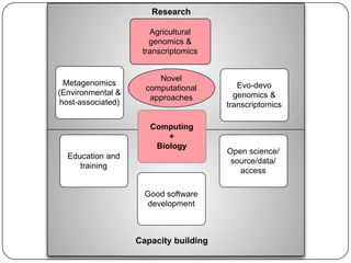
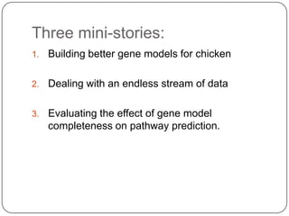
Three mini-stories are summarized from a document about genomics and bioinformatics in non-model organisms:
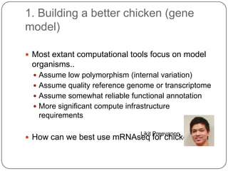
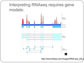
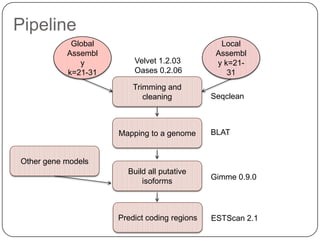
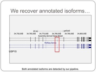
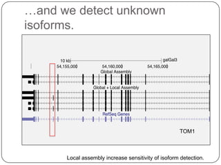
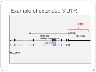
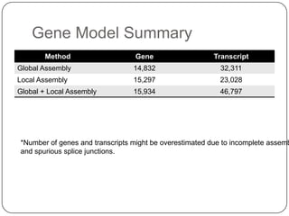
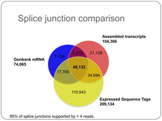
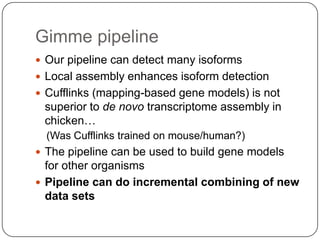
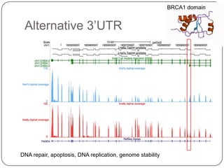
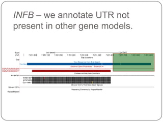
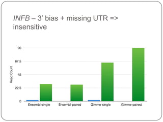
1. Building better gene models for the chicken genome using RNA-seq data helped recover annotated isoforms and detect unknown isoforms, resulting in over 15,000 genes and 46,000 transcripts identified.
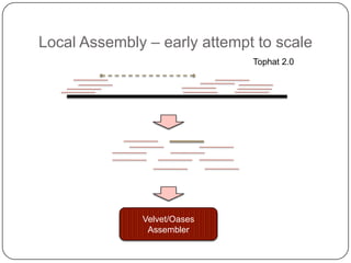
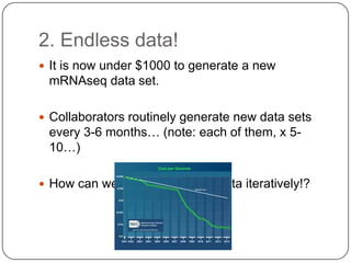
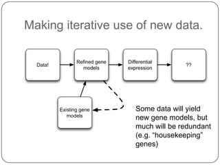
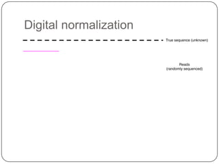
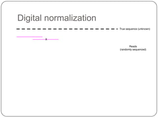
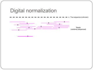
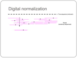
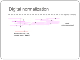
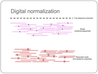
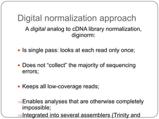
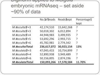
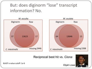
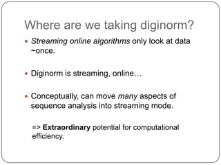
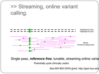
2. Digital normalization of sequencing data enabled iterative use of new data by setting aside 90% of redundant sequences, allowing analyses that would otherwise be impossible with limited computing resources.
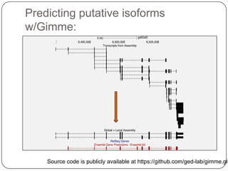
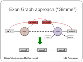
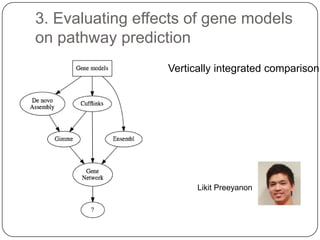
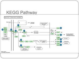
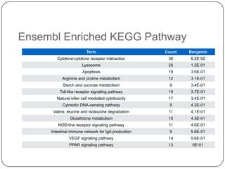
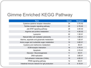
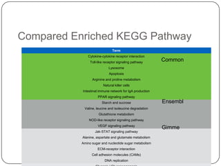
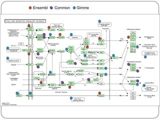
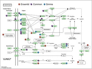
3. Comparing pathway predictions using Ensembl gene models versus gene models constructed with the Gimme pipeline showed both recovered known pathways but Gimme identified additional pathways, demonstrating effects of gene model completeness on downstream analyses.