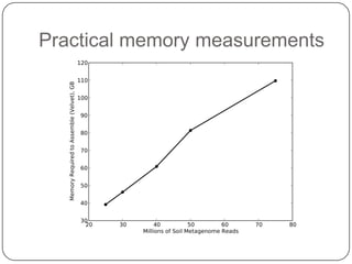
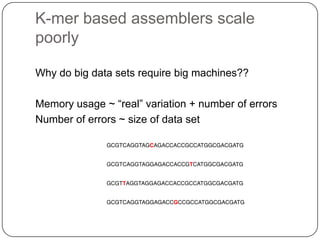
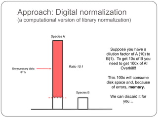
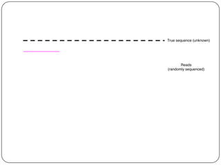
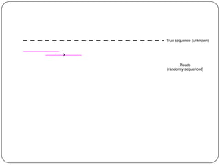
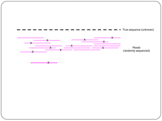
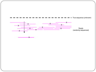
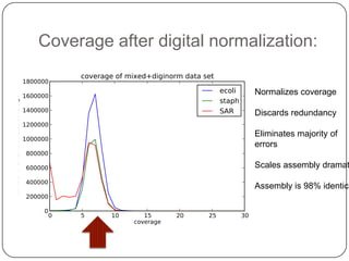
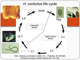
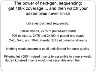
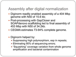
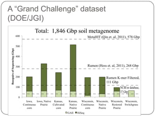
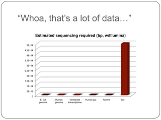
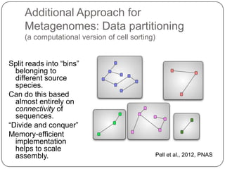
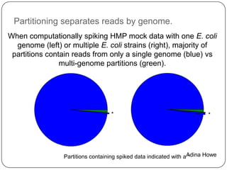
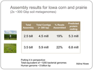
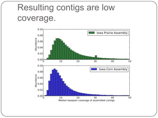
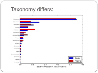
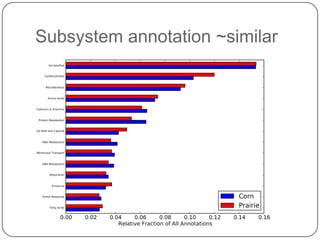
Building better genomes, transcriptomes, and
              metagenomes with improved
techniques for de novo assembly -- an easier way to do it

                    C. Titus Brown
                  Assistant Professor
                CSE, MMG, BEACON
               Michigan State University
                   December 2012
                    ctb@msu.edu
Acknowledgements
Lab members involved        Collaborators
   Adina Howe (w/Tiedje)    Jim Tiedje, MSU
   Jason Pell               Erich Schwarz, Caltech /
   Arend Hintze              Cornell
   Rosangela Canino-        Paul Sternberg, Caltech
    Koning                   Robin Gasser, U.
   Qingpeng Zhang            Melbourne
   Elijah Lowe              Weiming Li
   Likit Preeyanon         Funding
   Jiarong Guo
   Tim Brom                USDA NIFA; NSF IOS;
   Kanchan Pavangadkar          BEACON.
   Eric McDonald
We practice open science!
        “Be the change you want”

Everything discussed here:
 Code: github.com/ged-lab/ ; BSD license
 Blog: http://ivory.idyll.org/blog („titus brown blog‟)
 Twitter: @ctitusbrown
 Grants on Lab Web site:
  http://ged.msu.edu/interests.html
 Preprints: on arXiv, q-bio:
  „diginorm arxiv‟
My interests
I work primarily on organisms of agricultural,
evolutionary, or ecological importance, which tend
to have poor reference genomes and
transcriptomes. Focus on:

 Improving assembly sensitivity to better recover
 genomic/transcriptomic sequence, often from
 “weird” samples.

 Scaling sequence assembly approaches so that
 huge assemblies are possible and big assemblies
 are straightforward.
“Weird” biological samples:
 Single genome             Hard to sequence DNA
                              (e.g. GC/AT bias)

 Transcriptome             Differential expression!

 High polymorphism data    Multiple alleles

 Whole genome              Often extreme
 amplified                   amplification bias (next
                             slide)

 Metagenome (mixed         Differential abundance
 microbial community)        within community.
Shotgun sequencing and
coverage


 “Coverage” is simply the average number of reads that overlap
                  each true base in genome.

Here, the coverage is ~10 – just draw a line straight down from the
                  top through all of the reads.
Coverage plot of colony sequencing
vs single-cell amplification (MDA)


                               (MD amplified)
Non-normal coverage distributions
lead to decreased assembly
sensitivity
 Many assemblers embed a “coverage model” in
 their approach.
   Genome assemblers: abnormally low coverage is
    erroneous; abnormally high coverage is repetitive
    sequence.
   Transcriptome assemblers: isoforms should have
    same coverage across the entire isoform.
   Metagenome assemblers: differing abundances
    indicate different strains.


 Is there a different way? (Yes.)
Memory requirements (Velvet/Oases –
est)
 Bacterial genome      1-2 GB
 (colony)
                        500-1000 GB
 Human genome
                        100 GB +
 Vertebrate mRNA
                        100 GB
 Low complexity
 metagenome             1000 GB ++

 High complexity
 metagenome
Practical memory measurements
K-mer based assemblers scale
poorly

Why do big data sets require big machines??

Memory usage ~ “real” variation + number of errors
Number of errors ~ size of data set
Why does efficiency matter?
 It is now cheaper to generate sequence than it is
 to analyze it computationally!
   Machine time
   (Wo)man power/time


 More efficient programs allow better exploration
 of analysis parameters for maximizing sensitivity.

 Better or more sensitive bioinformatic approaches
 can be developed on top of more efficient theory.
Approach: Digital normalization
(a computational version of library normalization)


                                          Suppose you have a
                                       dilution factor of A (10) to
                                       B(1). To get 10x of B you
                                         need to get 100x of A!
                                                 Overkill!!

                                        This 100x will consume
                                       disk space and, because
                                          of errors, memory.

                                         We can discard it for
                                               you…
Digital normalization approach
   A digital analog to cDNA library normalization,
                       diginorm:

 Is single pass: looks at each read only once;


 Does not “collect” the majority of errors;


 Keeps all low-coverage reads;


 Smooths out coverage of regions.
Coverage before digital
normalization:


                          (MD amplified)
Coverage after digital normalization:

                            Normalizes coverage

                            Discards redundancy

                            Eliminates majority of
                            errors

                            Scales assembly dramat

                            Assembly is 98% identica
Digital normalization approach
   A digital analog to cDNA library normalization,
    diginorm is a read prefiltering approach that:

 Is single pass: looks at each read only once;


 Does not “collect” the majority of errors;


 Keeps all low-coverage reads;


 Smooths out coverage of regions.
Contig assembly is significantly more efficient and
now scales with underlying genome size


    Transcriptomes, microbial genomes incl MDA,
     and most metagenomes can be assembled in
     under 50 GB of RAM, with identical or improved
     results.
Some diginorm examples:

1.   Assembly of the H. contortus parasitic
     nematode genome, a “high polymorphism”
     problem.

2.   Reference-free assembly of the lamprey (P.
     marinus) transcriptome, a “big assembly”
     problem.

3.   Assembly of two Midwest soil metagenomes,
     Iowa corn and Iowa prairie – the “impossible”
     assembly problem.
1. The H. contortus problem
 A sheep parasite.


 ~350 Mbp genome


 Sequenced DNA 6 individuals after whole
 genome amplification, estimated 10%
 heterozygosity (!?)

 Significant bacterial contamination.


    (w/Robin Gasser, Paul Sternberg, and Erich
                    Schwarz)
H. contortus life cycle


Refs.: Nikolaou and Gasser (2006), Int. J. Parasitol. 36, 859-868;
        Prichard and Geary (2008), Nature 452, 157-158.
The power of next-gen. sequencing:
   get 180x coverage ... and then watch your
            assemblies never finish

                Libraries built and sequenced:

           300-nt inserts, 2x75 nt paired-end reads
     500-nt inserts, 2x75 and 2x100 nt paired-end reads
   2-kb, 5-kb, and 10-kb inserts, 2x49 nt paired-end reads

 Nothing would assemble at all until filtered for basic quality.

Filtering let ≤500 nt-sized inserts to assemble in a mere week.
But 2+ kb-sized inserts would not assemble even then.
Assembly after digital normalization
 Diginorm readily enabled assembly of a 404 Mbp
  genome with N50 of 15.6 kb;
 Post-processing with GapCloser and
  SOAPdenovo scaffolding led to final assembly of
  453 Mbp with N50 of 34.2kb.
 CEGMA estimates 73-94% complete genome.


 Diginorm helped by:
   Suppressing high polymorphism, esp in repeats;
   Eliminating 95% of sequencing errors;
   “Squashing” coverage variation from whole genome
   amplification and bacterial contamination
Next steps with H. contortus
 Publish the genome paper 


 Identification of antibiotic targets for treatment in
  agricultural settings (animal husbandry).

 Serving as “reference approach” for a wide
  variety of parasitic nematodes, many of which
  have similar genomic issues.
2. Lamprey transcriptome assembly.
 Lamprey genome is draft and missing ~30%.
 No closely related reference.
 Full-length and exon-level gene predictions are
 50-75% reliable, and rarely capture UTRs /
 isoforms.

 De novo assembly, if we do it well, can identify
   Novel genes
   Novel exons
   Fast evolving genes


 Somatic recombination: how much are we
 missing, really?
Sea lamprey in the Great Lakes


                 Non-native
                 Parasite of
                  medium to large
                  fishes
                 Caused
                  populations of
                  host fishes to
                  crash


                        Li Lab / Y-W C-D
Transcriptome results
 Started with 5.1 billion reads from 50 different
 tissues.

 Digital normalization discarded 98.7% of them as
 redundant, leaving 87m (!)

 These assembled into 15,100 transcripts > 1kb


 Against known transcripts, 98.7% agreement
 (accuracy); 99.7% included (contiguity)
Next steps with lamprey
 Far more complete transcriptome than the one
 predicted from the genome!

 Enabling studies in –
   Basal vertebrate phylogeny
   Biliary atresia
   Evolutionary origin of brown fat (previously thought
    to be mammalian only!)
   Pheromonal response in adults
3. Soil metagenome assembly
 Observation that 99% of microbes cannot easily
  be cultured in the lab. (“The great plate count
  anomaly”)
 Many reasons why you can‟t or don‟t want to
  culture:
   Syntrophic relationships
   Niche-specificity or unknown physiology
   Dormant microbes
   Abundance within communities


   Single-cell sequencing & shotgun metagenomics
      are two common ways to investigate microbial
                      communities.
SAMPLING LOCATIONS
Investigating soil microbial
ecology
 What ecosystem level functions are present, and
  how do microbes do them?
 How does agricultural soil differ from native soil?
 How does soil respond to climate perturbation?


 Questions that are not easy to answer without
 shotgun sequencing:
   What kind of strain-level heterogeneity is present in
    the population?
   What does the phage and viral population look like?
   What species are where?
A “Grand Challenge” dataset
(DOE/JGI)
                                               Total: 1,846 Gbp soil metagenome
                                600                                                       MetaHIT (Qin et. al, 2011), 578 Gbp

                                500
Basepairs of Sequencing (Gbp)


                                400


                                300                                                       Rumen (Hess et. al, 2011), 268 Gbp


                                200                                                                    Rumen K-mer Filtered,
                                                                                                       111 Gbp
                                100                                                                               NCBI nr database,
                                                                                                                  37 Gbp
                                  0
                                        Iowa,    Iowa, Native Kansas,      Kansas,   Wisconsin, Wisconsin, Wisconsin, Wisconsin,
                                      Continuous    Prairie   Cultivated   Native    Continuous  Native    Restored Switchgrass
                                         corn                   corn       Prairie     corn      Prairie    Prairie
                                                                           GAII   HiSeq
“Whoa, that‟s a lot of data…”
           Estimated sequencing required (bp, w/Illumina)

  5E+14

 4.5E+14

  4E+14

 3.5E+14

  3E+14

 2.5E+14

  2E+14

 1.5E+14

  1E+14

  5E+13

      0
             E. coli   Human      Vertebrate    Human gut   Marine   Soil
            genome     genome   transcriptome
Additional Approach for
     Metagenomes: Data partitioning
     (a computational version of cell sorting)


Split reads into “bins”
  belonging to
  different source
  species.
Can do this based
  almost entirely on
  connectivity of
  sequences.
“Divide and conquer”
Memory-efficient
  implementation
  helps to scale
  assembly.                                      Pell et al., 2012, PNAS
Partitioning separates reads by genome.
When computationally spiking HMP mock data with one E. coli
  genome (left) or multiple E. coli strains (right), majority of
 partitions contain reads from only a single genome (blue) vs
                multi-genome partitions (green).


                                   *                                     *


                 Partitions containing spiked data indicated with aAdina Howe
                                                                   *
Assembly results for Iowa corn and prairie
(2x ~300 Gbp soil metagenomes)


                                                    Predicted
          Total     Total Contigs    % Reads
                                                     protein
        Assembly     (> 300 bp)     Assembled
                                                     coding


        2.5 bill      4.5 mill         19%          5.3 mill


        3.5 bill      5.9 mill         22%          6.8 mill


      Putting it in perspective:
      Total equivalent of ~1200 bacterial genomes         Adina Howe
      Human genome ~3 billion bp
Resulting contigs are low
coverage.


   Figure 11: Coverage (median basepair) dist ribut ion of assembled cont igs from soil met agenomes.
Strain variation?
                                                             Can measure
                                                             by read
Top two allele frequencies


                                                             mapping.
                                                             Of 5000 most
                                                             abundant
                                                             contigs, only 1
                                                             has a
                                                             polymorphism
                                                             rate > 5%


                                    Position within contig
Tentative observations from our soil
samples:
 We need 100x as much data…
 A lot of our sample may consist of phage.
 Phylogeny varies more than functional
  predictions.
 We see little to no strain variation within our
  samples
   Not bulk soil!
   Very small, localized, and low coverage samples
 We may be able to do selective really deep
  sequencing and then infer the rest from 16s.
   Implications for soil aggregate assembly?
Some concluding thoughts
 Digital normalization is a very powerful technique
  for “fixing” weird samples. (…and all samples are
  weird.)
 A number of real world projects are using
  diginorm successfully (~6-10 in my lab; ~30-40?
  overall).
 A diginorm-derived procedure is now a
  recommended part of the Trinity mRNAseq
  assembler.

 Diginorm is
  1. Very computationally efficient;
  2. Always “cheaper” than running an assembler in
     the first place
Where next?
 Assembly in the cloud!

 Study and formalize paired/end mate pair handling in
  diginorm.

 Web interface to run and evaluate assemblies.

 New methods to evaluate and improve
  assemblies, including a “meta assembly” approach for
  metagenomes.

 Fast and efficient error correction of sequencing data
   Can also address assembly of high polymorphism
    sequence, allelic mapping bias, and others;
   Can also enable fast/efficient storage and search of nucleic
    acid databases.
Four+ papers on our work, soon.
 2012 PNAS, Pell et al., pmid 22847406
 (partitioning).

 In review, Brown et al., arXiv:1203.4802 (digital
 normalization).

 Submitted, Howe et al, arXiv: 1212.0159 (artifact
 removal from Illumina metagenomes).

 In preparation, Howe et al. – assembling the heck
 out of soil.

 In preparation, Zhang et al. – efficient k-mer
Education: next-gen sequence
course
    June 2013, Kellogg Biological Station; < $500
     Hands on exposure to data, analysis tools.


 Metagenomics workshop HERE, tomorrow, 9am-3pm – contact Lex Nederbra
Thanks!

Everything discussed here:
 Code: github.com/ged-lab/ ; BSD license
 Blog: http://ivory.idyll.org/blog („titus brown blog‟)
 Twitter: @ctitusbrown
 Grants on Lab Web site:
  http://ged.msu.edu/interests.html
 Preprints: on arXiv, q-bio:
  „diginorm arxiv‟
Why are we applying short-read sequencing to
RNAseq and metagenomics?
 Short-read sampling is deep and quantitative.
   Statistical argument: your ability to observe rare
    sequences – your sensitivity of measurement – is
    directly related to the number of independent
    sequences you take.
   Longer reads (PacBio, 454, Ion Torrent) are less
    informative for quantitation.


 Majority of metagenome studies going forward
 will make use of Illumina (~2-3 year statement 
Digital normalization retains information, while
discarding data and errors
Lossy compression


                    http://en.wikipedia.org/wiki/JPEG
Lossy compression


                    http://en.wikipedia.org/wiki/JPEG
Lossy compression


                    http://en.wikipedia.org/wiki/JPEG
Lossy compression


                    http://en.wikipedia.org/wiki/JPEG
Lossy compression


                    http://en.wikipedia.org/wiki/JPEG

2012 oslo-talk

  • 1.
    Building better genomes,transcriptomes, and metagenomes with improved techniques for de novo assembly -- an easier way to do it C. Titus Brown Assistant Professor CSE, MMG, BEACON Michigan State University December 2012 ctb@msu.edu
  • 2.
    Acknowledgements Lab members involved Collaborators  Adina Howe (w/Tiedje)  Jim Tiedje, MSU  Jason Pell  Erich Schwarz, Caltech /  Arend Hintze Cornell  Rosangela Canino-  Paul Sternberg, Caltech Koning  Robin Gasser, U.  Qingpeng Zhang Melbourne  Elijah Lowe  Weiming Li  Likit Preeyanon Funding  Jiarong Guo  Tim Brom USDA NIFA; NSF IOS;  Kanchan Pavangadkar BEACON.  Eric McDonald
  • 3.
    We practice openscience! “Be the change you want” Everything discussed here:  Code: github.com/ged-lab/ ; BSD license  Blog: http://ivory.idyll.org/blog („titus brown blog‟)  Twitter: @ctitusbrown  Grants on Lab Web site: http://ged.msu.edu/interests.html  Preprints: on arXiv, q-bio: „diginorm arxiv‟
  • 5.
    My interests I workprimarily on organisms of agricultural, evolutionary, or ecological importance, which tend to have poor reference genomes and transcriptomes. Focus on:  Improving assembly sensitivity to better recover genomic/transcriptomic sequence, often from “weird” samples.  Scaling sequence assembly approaches so that huge assemblies are possible and big assemblies are straightforward.
  • 6.
    “Weird” biological samples: Single genome  Hard to sequence DNA (e.g. GC/AT bias)  Transcriptome  Differential expression!  High polymorphism data  Multiple alleles  Whole genome  Often extreme amplified amplification bias (next slide)  Metagenome (mixed  Differential abundance microbial community) within community.
  • 7.
    Shotgun sequencing and coverage “Coverage” is simply the average number of reads that overlap each true base in genome. Here, the coverage is ~10 – just draw a line straight down from the top through all of the reads.
  • 8.
    Coverage plot ofcolony sequencing vs single-cell amplification (MDA) (MD amplified)
  • 9.
    Non-normal coverage distributions leadto decreased assembly sensitivity  Many assemblers embed a “coverage model” in their approach.  Genome assemblers: abnormally low coverage is erroneous; abnormally high coverage is repetitive sequence.  Transcriptome assemblers: isoforms should have same coverage across the entire isoform.  Metagenome assemblers: differing abundances indicate different strains.  Is there a different way? (Yes.)
  • 10.
    Memory requirements (Velvet/Oases– est)  Bacterial genome  1-2 GB (colony)  500-1000 GB  Human genome  100 GB +  Vertebrate mRNA  100 GB  Low complexity metagenome  1000 GB ++  High complexity metagenome
  • 11.
  • 12.
    K-mer based assemblersscale poorly Why do big data sets require big machines?? Memory usage ~ “real” variation + number of errors Number of errors ~ size of data set
  • 13.
    Why does efficiencymatter?  It is now cheaper to generate sequence than it is to analyze it computationally!  Machine time  (Wo)man power/time  More efficient programs allow better exploration of analysis parameters for maximizing sensitivity.  Better or more sensitive bioinformatic approaches can be developed on top of more efficient theory.
  • 14.
    Approach: Digital normalization (acomputational version of library normalization) Suppose you have a dilution factor of A (10) to B(1). To get 10x of B you need to get 100x of A! Overkill!! This 100x will consume disk space and, because of errors, memory. We can discard it for you…
  • 21.
    Digital normalization approach A digital analog to cDNA library normalization, diginorm:  Is single pass: looks at each read only once;  Does not “collect” the majority of errors;  Keeps all low-coverage reads;  Smooths out coverage of regions.
  • 22.
  • 23.
    Coverage after digitalnormalization: Normalizes coverage Discards redundancy Eliminates majority of errors Scales assembly dramat Assembly is 98% identica
  • 24.
    Digital normalization approach A digital analog to cDNA library normalization, diginorm is a read prefiltering approach that:  Is single pass: looks at each read only once;  Does not “collect” the majority of errors;  Keeps all low-coverage reads;  Smooths out coverage of regions.
  • 25.
    Contig assembly issignificantly more efficient and now scales with underlying genome size  Transcriptomes, microbial genomes incl MDA, and most metagenomes can be assembled in under 50 GB of RAM, with identical or improved results.
  • 26.
    Some diginorm examples: 1. Assembly of the H. contortus parasitic nematode genome, a “high polymorphism” problem. 2. Reference-free assembly of the lamprey (P. marinus) transcriptome, a “big assembly” problem. 3. Assembly of two Midwest soil metagenomes, Iowa corn and Iowa prairie – the “impossible” assembly problem.
  • 27.
    1. The H.contortus problem  A sheep parasite.  ~350 Mbp genome  Sequenced DNA 6 individuals after whole genome amplification, estimated 10% heterozygosity (!?)  Significant bacterial contamination. (w/Robin Gasser, Paul Sternberg, and Erich Schwarz)
  • 28.
    H. contortus lifecycle Refs.: Nikolaou and Gasser (2006), Int. J. Parasitol. 36, 859-868; Prichard and Geary (2008), Nature 452, 157-158.
  • 29.
    The power ofnext-gen. sequencing: get 180x coverage ... and then watch your assemblies never finish Libraries built and sequenced: 300-nt inserts, 2x75 nt paired-end reads 500-nt inserts, 2x75 and 2x100 nt paired-end reads 2-kb, 5-kb, and 10-kb inserts, 2x49 nt paired-end reads Nothing would assemble at all until filtered for basic quality. Filtering let ≤500 nt-sized inserts to assemble in a mere week. But 2+ kb-sized inserts would not assemble even then.
  • 30.
    Assembly after digitalnormalization  Diginorm readily enabled assembly of a 404 Mbp genome with N50 of 15.6 kb;  Post-processing with GapCloser and SOAPdenovo scaffolding led to final assembly of 453 Mbp with N50 of 34.2kb.  CEGMA estimates 73-94% complete genome.  Diginorm helped by:  Suppressing high polymorphism, esp in repeats;  Eliminating 95% of sequencing errors;  “Squashing” coverage variation from whole genome amplification and bacterial contamination
  • 31.
    Next steps withH. contortus  Publish the genome paper   Identification of antibiotic targets for treatment in agricultural settings (animal husbandry).  Serving as “reference approach” for a wide variety of parasitic nematodes, many of which have similar genomic issues.
  • 32.
    2. Lamprey transcriptomeassembly.  Lamprey genome is draft and missing ~30%.  No closely related reference.  Full-length and exon-level gene predictions are 50-75% reliable, and rarely capture UTRs / isoforms.  De novo assembly, if we do it well, can identify  Novel genes  Novel exons  Fast evolving genes  Somatic recombination: how much are we missing, really?
  • 33.
    Sea lamprey inthe Great Lakes  Non-native  Parasite of medium to large fishes  Caused populations of host fishes to crash Li Lab / Y-W C-D
  • 34.
    Transcriptome results  Startedwith 5.1 billion reads from 50 different tissues.  Digital normalization discarded 98.7% of them as redundant, leaving 87m (!)  These assembled into 15,100 transcripts > 1kb  Against known transcripts, 98.7% agreement (accuracy); 99.7% included (contiguity)
  • 35.
    Next steps withlamprey  Far more complete transcriptome than the one predicted from the genome!  Enabling studies in –  Basal vertebrate phylogeny  Biliary atresia  Evolutionary origin of brown fat (previously thought to be mammalian only!)  Pheromonal response in adults
  • 36.
    3. Soil metagenomeassembly  Observation that 99% of microbes cannot easily be cultured in the lab. (“The great plate count anomaly”)  Many reasons why you can‟t or don‟t want to culture:  Syntrophic relationships  Niche-specificity or unknown physiology  Dormant microbes  Abundance within communities Single-cell sequencing & shotgun metagenomics are two common ways to investigate microbial communities.
  • 37.
  • 38.
    Investigating soil microbial ecology What ecosystem level functions are present, and how do microbes do them?  How does agricultural soil differ from native soil?  How does soil respond to climate perturbation?  Questions that are not easy to answer without shotgun sequencing:  What kind of strain-level heterogeneity is present in the population?  What does the phage and viral population look like?  What species are where?
  • 39.
    A “Grand Challenge”dataset (DOE/JGI) Total: 1,846 Gbp soil metagenome 600 MetaHIT (Qin et. al, 2011), 578 Gbp 500 Basepairs of Sequencing (Gbp) 400 300 Rumen (Hess et. al, 2011), 268 Gbp 200 Rumen K-mer Filtered, 111 Gbp 100 NCBI nr database, 37 Gbp 0 Iowa, Iowa, Native Kansas, Kansas, Wisconsin, Wisconsin, Wisconsin, Wisconsin, Continuous Prairie Cultivated Native Continuous Native Restored Switchgrass corn corn Prairie corn Prairie Prairie GAII HiSeq
  • 40.
    “Whoa, that‟s alot of data…” Estimated sequencing required (bp, w/Illumina) 5E+14 4.5E+14 4E+14 3.5E+14 3E+14 2.5E+14 2E+14 1.5E+14 1E+14 5E+13 0 E. coli Human Vertebrate Human gut Marine Soil genome genome transcriptome
  • 41.
    Additional Approach for Metagenomes: Data partitioning (a computational version of cell sorting) Split reads into “bins” belonging to different source species. Can do this based almost entirely on connectivity of sequences. “Divide and conquer” Memory-efficient implementation helps to scale assembly. Pell et al., 2012, PNAS
  • 42.
    Partitioning separates readsby genome. When computationally spiking HMP mock data with one E. coli genome (left) or multiple E. coli strains (right), majority of partitions contain reads from only a single genome (blue) vs multi-genome partitions (green). * * Partitions containing spiked data indicated with aAdina Howe *
  • 43.
    Assembly results forIowa corn and prairie (2x ~300 Gbp soil metagenomes) Predicted Total Total Contigs % Reads protein Assembly (> 300 bp) Assembled coding 2.5 bill 4.5 mill 19% 5.3 mill 3.5 bill 5.9 mill 22% 6.8 mill Putting it in perspective: Total equivalent of ~1200 bacterial genomes Adina Howe Human genome ~3 billion bp
  • 44.
    Resulting contigs arelow coverage. Figure 11: Coverage (median basepair) dist ribut ion of assembled cont igs from soil met agenomes.
  • 45.
    Strain variation? Can measure by read Top two allele frequencies mapping. Of 5000 most abundant contigs, only 1 has a polymorphism rate > 5% Position within contig
  • 46.
    Tentative observations fromour soil samples:  We need 100x as much data…  A lot of our sample may consist of phage.  Phylogeny varies more than functional predictions.  We see little to no strain variation within our samples  Not bulk soil!  Very small, localized, and low coverage samples  We may be able to do selective really deep sequencing and then infer the rest from 16s.  Implications for soil aggregate assembly?
  • 47.
    Some concluding thoughts Digital normalization is a very powerful technique for “fixing” weird samples. (…and all samples are weird.)  A number of real world projects are using diginorm successfully (~6-10 in my lab; ~30-40? overall).  A diginorm-derived procedure is now a recommended part of the Trinity mRNAseq assembler.  Diginorm is 1. Very computationally efficient; 2. Always “cheaper” than running an assembler in the first place
  • 48.
    Where next?  Assemblyin the cloud!  Study and formalize paired/end mate pair handling in diginorm.  Web interface to run and evaluate assemblies.  New methods to evaluate and improve assemblies, including a “meta assembly” approach for metagenomes.  Fast and efficient error correction of sequencing data  Can also address assembly of high polymorphism sequence, allelic mapping bias, and others;  Can also enable fast/efficient storage and search of nucleic acid databases.
  • 49.
    Four+ papers onour work, soon.  2012 PNAS, Pell et al., pmid 22847406 (partitioning).  In review, Brown et al., arXiv:1203.4802 (digital normalization).  Submitted, Howe et al, arXiv: 1212.0159 (artifact removal from Illumina metagenomes).  In preparation, Howe et al. – assembling the heck out of soil.  In preparation, Zhang et al. – efficient k-mer
  • 50.
    Education: next-gen sequence course June 2013, Kellogg Biological Station; < $500 Hands on exposure to data, analysis tools. Metagenomics workshop HERE, tomorrow, 9am-3pm – contact Lex Nederbra
  • 51.
    Thanks! Everything discussed here: Code: github.com/ged-lab/ ; BSD license  Blog: http://ivory.idyll.org/blog („titus brown blog‟)  Twitter: @ctitusbrown  Grants on Lab Web site: http://ged.msu.edu/interests.html  Preprints: on arXiv, q-bio: „diginorm arxiv‟
  • 53.
    Why are weapplying short-read sequencing to RNAseq and metagenomics?  Short-read sampling is deep and quantitative.  Statistical argument: your ability to observe rare sequences – your sensitivity of measurement – is directly related to the number of independent sequences you take.  Longer reads (PacBio, 454, Ion Torrent) are less informative for quantitation.  Majority of metagenome studies going forward will make use of Illumina (~2-3 year statement 
  • 54.
    Digital normalization retainsinformation, while discarding data and errors
  • 55.
    Lossy compression http://en.wikipedia.org/wiki/JPEG
  • 56.
    Lossy compression http://en.wikipedia.org/wiki/JPEG
  • 57.
    Lossy compression http://en.wikipedia.org/wiki/JPEG
  • 58.
    Lossy compression http://en.wikipedia.org/wiki/JPEG
  • 59.
    Lossy compression http://en.wikipedia.org/wiki/JPEG

Editor's Notes

  • #26 Goal is to do first stage data reduction/analysis in less time than it takes to generate the data. Compression =&gt; OLC assembly.
  • #34 Larvae/stream bottoms 3-6 years; parasitic adult -&gt; great lakes, 12-20 months feeding. 5-8 years. 40 lbs of fish per life as parasite. 98% of fish in great lakes went away!
  • #46 Diginorm is a subsampling approach that may help assemble highly polymorphic sequences. Observed levels of variation are quite low relative to e.g. marine free spawning animals.