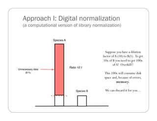
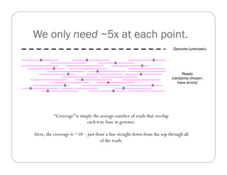
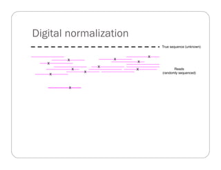
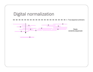
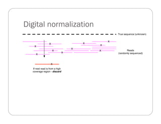
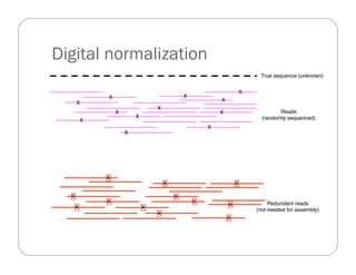
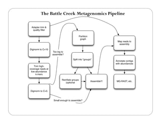
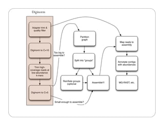
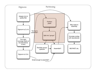
C.Titus Brown
Assistant Professor
CSE, MMG, BEACON
Michigan State University
August 2013
ctb@msu.edu
Assembling metagenomes: a not so practical guide
Acknowledgements
Lab members involved Collaborators
—  Adina Howe (w/Tiedje)
—  Jason Pell
—  Arend Hintze
—  Rosangela Canino-Koning
—  Qingpeng Zhang
—  Elijah Lowe
—  Likit Preeyanon
—  Jiarong Guo
—  Tim Brom
—  Kanchan Pavangadkar
—  Eric McDonald
—  JimTiedje, MSU; Janet
Jansson, JGI; Susannah
Tringe, JGI.
Funding
USDA NIFA; NSF IOS;
BEACON, NIH.
Shotgun sequencing and coverage
Genome (unknown)
X
X
X
X
X
X
X
X
X
X
X
X
X
X
Reads
(randomly chosen;
have errors)
X
XX
“Coverage” is simply the average number of reads that overlap
each true base in genome.
Here, the coverage is ~10 – just draw a line straight down from the top through all
of the reads.
Random sampling => deep sampling
needed
Typically 10-100x needed for robust recovery (300 Gbp for human)
Coverage distribution matters!
(MD amplified)
Assembly depends on high coverage
Shared low-level
transcripts may not
reach the threshold
for assembly.
K-mer based assemblers scale poorly
Why do big data sets require big machines??
Memory usage ~ “real” variation + number of errors
Number of errors ~ size of data set
GCGTCAGGTAGGAGACCGCCGCCATGGCGACGATG
GCGTCAGGTAGGAGACCACCGTCATGGCGACGATG
GCGTCAGGTAGCAGACCACCGCCATGGCGACGATG
GCGTTAGGTAGGAGACCACCGCCATGGCGACGATG
Conway T C , Bromage A J Bioinformatics 2011;27:479-486
© The Author 2011. Published by Oxford University Press. All rights reserved. For Permissions,
please email: journals.permissions@oup.com
De Bruijn graphs scale poorly with data size
Practical memory measurements
Velvet measurements (Adina Howe)
How much data do we need? (I)
(“More” is rather vague…)
Putting it in perspective:
Total equivalent of ~1200 bacterial genomes
Human genome ~3 billion bp
Assembly results for Iowa corn and prairie
(2x ~300 Gbp soil metagenomes)
Total
Assembly
Total Contigs
(> 300 bp)
% Reads
Assembled
Predicted
protein
coding
2.5 bill 4.5 mill 19% 5.3 mill
3.5 bill 5.9 mill 22% 6.8 mill
Adina Howe
Resulting contigs are low coverage.
Figure 11: Coverage (median basepair) distribution of assembled contigs from soil metagenomes.
How much? (II)
—  Suppose we need 10x coverage to assemble a microbial
genome, and microbial genomes average 5e6 bp of DNA.
—  Further suppose that we want to be able to assemble a
microbial species that is “1 in a 100000”, i.e. 1 in 1e5.
—  Shotgun sequencing samples randomly, so must sample deeply
to be sensitive.
10x coverage x 5e6 bp x 1e5 =~ 50e11, or 5 Tbp of sequence.
Currently this would cost approximately $100k, for 10 full
Illumina runs, but in a year we will be able to do it for much
less.
We can estimate sequencing req’d:
http://ivory.idyll.org/blog/how-much-sequencing-is-needed.html
“Whoa, that’s a lot of data…”
http://ivory.idyll.org/blog/how-much-sequencing-is-needed.html
Some approximate metagenome sizes
—  Deep carbon mine data set: 60 Mbp (x 10x => 600 Mbp)
—  Great Prairie soil: 12 Gbp (4x human genome)
—  Amazon Rain Forest Microbial Observatory soil: 26 Gbp
How can we scale assembly!?
—  We have developed two prefiltering approaches.
—  Essentially, we preprocess your reads and (a) normalize their
coverage and (b) subdivide them by graph partition.
“We take your reads and make them better! Satisfaction guaranteed or your
money back!*”
*Terms may not apply to NSF, NIH, and USDA funding bodies.
Approach I: Digital normalization
(a computational version of library normalization)
Species A
Species B
Ratio 10:1
Unnecessary data
81%
Suppose you have a dilution
factor ofA (10) to B(1). To get
10x of B you need to get 100x
ofA! Overkill!!
This 100x will consume disk
space and, because of errors,
memory.
We can discard it for you…
We only need ~5x at each point.
Genome (unknown)
X
X
X
X
X
X
X
X
X
X
X
X
X
X
Reads
(randomly chosen;
have errors)
X
XX
“Coverage” is simply the average number of reads that overlap
each true base in genome.
Here, the coverage is ~10 – just draw a line straight down from the top through all
of the reads.
True sequence (unknown)
Reads
(randomly sequenced)
Digital normalization
True sequence (unknown)
Reads
(randomly sequenced)
X
Digital normalization
True sequence (unknown)
Reads
(randomly sequenced)
X
X
X
X
X
X
X
X
X
X
X
Digital normalization
True sequence (unknown)
Reads
(randomly sequenced)
X
X
X
X
X
X
X
X
X
X
X
Digital normalization
True sequence (unknown)
Reads
(randomly sequenced)
X
X
X
X
X
X
X
X
X
If next read is from a high
coverage region - discard
X
X
Digital normalization
True sequence (unknown)
Reads
(randomly sequenced)
X
X
X
X
X
X
X
X
X
X
X
X
X
X
X
X
X
X
X
X
X
X
X
X
Redundant reads
(not needed for assembly)
A read’s median k-mer count is a good
estimator of “coverage”.
This gives us a
reference-free
measure of coverage.
Digital normalization approach
A digital analog to cDNA library normalization, diginorm:
—  Is single pass: looks at each read only once;
—  Does not “collect” the majority of errors;
—  Keeps all low-coverage reads;
—  Smooths out coverage of regions.
Coverage before digital normalization:
(MD amplified)
Coverage after digital normalization:
Normalizes coverage
Discards redundancy
Eliminates majority of
errors
Scales assembly dramatically.
Assembly is 98% identical.
Digital normalization approach
A digital analog to cDNA library normalization, diginorm is a
read prefiltering approach that:
—  Is single pass: looks at each read only once;
—  Does not “collect” the majority of errors;
—  Keeps all low-coverage reads;
—  Smooths out coverage of regions.
Contig assembly is significantly more efficient and now
scales with underlying genome size
—  Transcriptomes, microbial genomes incl MDA, and most
metagenomes can be assembled in under 50 GB of RAM,
with identical or improved results.
Digital normalization retains information, while
discarding data and errors
http://en.wikipedia.org/wiki/JPEG
Lossy compression
http://en.wikipedia.org/wiki/JPEG
Lossy compression
http://en.wikipedia.org/wiki/JPEG
Lossy compression
http://en.wikipedia.org/wiki/JPEG
Lossy compression
http://en.wikipedia.org/wiki/JPEG
Lossy compression
Raw data
(~10-100 GB)
Analysis "Information"
~1 GB
"Information"
"Information"
"Information"
"Information"
Database &
integration
We can use lossy compression approaches to make downstream
analysis faster and better.
~2 GB – 2TB of single-chassis RAM
Metagenomes: Data partitioning
(a computational version of cell sorting)
Split reads into “bins”
belonging to different
source species.
Can do this based almost
entirely on connectivity of
sequences.
“Divide and conquer”
Memory-efficient
implementation helps to
scale assembly.
Pell et al., 2012, PNAS
Partitioning separates reads by genome.
When computationally spiking HMP mock data with one E.coli genome
(left) or multiple E.coli strains (right), majority of partitions contain reads
from only a single genome (blue) vs multi-genome partitions (green).
Partitions containing spiked data indicated with a * Adina Howe
**
Partitioning: Technical challenges met (and
defeated)
—  Novel data structure properties elucidated via percolation
theory analysis (Pell et al., 2012, PNAS).
—  Exhaustive in-memory traversal of graphs containing 5-15
billion nodes.
—  Sequencing technology introduces false sequences in graph
(Howe et al., submitted.)
—  Only 20x improvement in assembly scaling L.
Is your assembly good?
—  Truly reference-free assembly is hard to evaluate.
—  Traditional “genome” measures like N50 and NG50 simply do
not apply to metagenomes, because very often you don’t
know what the genome “size” is.
Evaluating assembly
Predicted genome.
X
X
X
X
X
X
X
X
XX
Reads - noisy observations
of some genome.
Assembler
(a Big Black Box)
Evaluating correctness of metagenomes is still undiscovered country.
Assembler overlap?
See tutorial.
What’s the best assembler?
-25
-20
-15
-10
-5
0
5
10
BCM* BCM ALLP NEWB SOAP** MERAC CBCB SOAP* SOAP SGA PHUS RAY MLK ABL
CumulativeZ-scorefromrankingmetrics
Bird assembly
Bradnam et al.,Assemblathon 2:
http://arxiv.org/pdf/1301.5406v1.pdf
What’s the best assembler?
-8
-6
-4
-2
0
2
4
6
8
BCM CSHL CSHL* SYM ALLP SGA SOAP* MERAC ABYSS RAY IOB CTD IOB* CSHL** CTD** CTD*
CumulativeZ-scorefromrankingmetrics
Fish assembly
Bradnam et al.,Assemblathon 2:
http://arxiv.org/pdf/1301.5406v1.pdf
What’s the best assembler?
Bradnam et al.,Assemblathon 2:
http://arxiv.org/pdf/1301.5406v1.pdf
-14
-10
-6
-2
2
6
10
SGA PHUS MERAC SYMB ABYSS CRACS BCM RAY SOAP GAM CURT
CumulativeZ-scorefromrankingmetrics
Snake assembly
Answer: for eukaryotic genomes, it
depends
—  Different assemblers perform differently, depending on
—  Repeat content
—  Heterozygosity
—  Generally the results are very good (est completeness, etc.)
but different between different assemblers (!)
—  There Is No OneAnswer.
Estimated completeness: CEGMA
Each assembler lost different ~5% CEGs
Bradnam et al.,Assemblathon 2:
http://arxiv.org/pdf/1301.5406v1.pdf
Tradeoffs in N 50 and % incl.
0
10
20
30
40
50
60
70
80
90
100
110
0
2,000,000
4,000,000
6,000,000
8,000,000
10,000,000
12,000,000
14,000,000
16,000,000
18,000,000
BCM ALLP SOAP NEWB MERAC SGA CBCB PHUS RAY MLK ABL
%ofestimatedgenomesizepresentinscaffolds>=25Kbp
NG50scaffoldlength(bp)
Bird assembly
Bradnam et al.,Assemblathon 2:
http://arxiv.org/pdf/1301.5406v1.pdf
Evaluating assemblies
—  Every assembly returns different results for eukaryotic genomes.
—  For metagenomes, it’s even worse.
—  No systematic exploration of precision, recall, etc.
—  Very little in the way of cross-comparable data sets
—  Often sequencing technology being evaluated is out of date
—  etc. etc.
Our experience
—  Our metagenome assemblies compare well with others, but
we have little in the way of ground truth with which to
evaluate.
—  Scaffold assembly is tricky; we believe in contig assembly for
metagenomes, but not scaffolding.
—  See arXiv paper,“Assembling large, complex metagenomes”,
for our suggested pipeline and statistics & references.
Metagenomic assemblies are highly variable
Adina Howe et al., arXiv 1212.0159
How to choose a metagenome
assembler
—  Try a few.
—  Use what seems to perform best (most bp > some
minimum)
—  I’ve heard/read good things about
—  MetaVelvet
—  Ray Meta
—  IDBA-UD
—  Our pipeline doesn’t specify an assembler.
Adapter trim &
quality filter
Diginorm to C=10
Trim high-
coverage reads at
low-abundance
k-mers
Diginorm to C=5
Partition
graph
Split into "groups"
Reinflate groups
(optional
Assemble!!!
Map reads to
assembly
Too big to
assemble?
Small enough to assemble?
Annotate contigs
with abundances
MG-RAST, etc.
The Battle Creek Metagenomics Pipeline
Adapter trim &
quality filter
Diginorm to C=10
Trim high-
coverage reads at
low-abundance
k-mers
Diginorm to C=5
Partition
graph
Split into "groups"
Reinflate groups
(optional
Assemble!!!
Map reads to
assembly
Too big to
assemble?
Small enough to assemble?
Annotate contigs
with abundances
MG-RAST, etc.
Diginorm
Adapter trim &
quality filter
Diginorm to C=10
Trim high-
coverage reads at
low-abundance
k-mers
Diginorm to C=5
Partition
graph
Split into "groups"
Reinflate groups
(optional
Assemble!!!
Map reads to
assembly
Too big to
assemble?
Small enough to assemble?
Annotate contigs
with abundances
MG-RAST, etc.
Diginorm Partitioning
Thoughts on our pipeline
—  Should work with any metagenome; very generic approach.
—  Diginorm can be decoupled from partitioning;
—  People report that diginorm “just works”;
—  Partitioning is trickier and only needed for REALLY BIG data sets.
—  Diginorm does interact with some assemblers in a funny way, so
suggest starting withVelvet and/or reinflating your partitions.
—  This pipeline, esp diginorm part, is faster and lower memory than any
other assembler out there (well, except maybe Minia).
Deep Carbon data set
—  Name: DCO_TCO_MM5
—  Masimong Gold Mine; microbial cells filtered from fracture
water from within a 1.9km borehole. (32,000 year old
water?!)
—  M.C.Y. Lau, C. Magnabosco, S. Grim, G. Lacrampe
Couloume, K.Wilkie, B. Sherwood Lollar, D.N. Simkus, G.F.
Slater, S. Hendrickson, M. Pullin,T.L. Kieft, O. Kuloyo, B.
Linage, G. Borgonie, E. van Heerden, J.Ackerman, C. van
Jaarsveld, andT.C. Onstott
DCO_TCO_MM520m reads / 2.1 Gbp
5.6m reads / 601.3 Mbp
Adapter trim &
quality filter
Diginorm to C=10
Trim high-
coverage reads at
low-abundance
k-mers
“Could you take a look at this? MG-
RAST is telling us we have a lot of
artificially duplicated reads, i.e. the
data is bad.”
Entire process took ~4 hours of
computation, or so.
(Minimum genome size est: 60.1 Mbp)
Assembly stats:
All	
  con'gs	
   Con'gs	
  >	
  1kb	
  
k	
   N	
  con'gs	
   Sum	
  BP	
   N	
  con'gs	
   Sum	
  BP	
  
Max	
  
con'g	
  
21	
   343263	
   63217837	
   6271	
   10537601	
   9987	
  
23	
   302613	
   63025311	
   7183	
   13867885	
   21348	
  
25	
   276261	
   62874727	
   7375	
   15303646	
   34272	
  
27	
   258073	
   62500739	
   7424	
   16078145	
   48742	
  
29	
   242552	
   62001315	
   7349	
   16426147	
   48746	
  
31	
   228043	
   61445912	
   7307	
   16864293	
   48750	
  
33	
   214559	
   60744478	
   7241	
   17133827	
   48768	
  
35	
   203292	
   60039871	
   7129	
   17249351	
   45446	
  
37	
   189948	
   58899828	
   7088	
   17527450	
   59437	
  
39	
   180754	
   58146806	
   7027	
   17610071	
   54112	
  
41	
   172209	
   57126650	
   6914	
   17551789	
   65207	
  
43	
   165563	
   56440648	
   6925	
   17654067	
   73231	
  
DCO_TCO_MM5
(Minimum genome size est: 60.1 Mbp)
Chose two:
—  A: k=43 (“long contigs”)
—  165563 contigs
—  56.4 Mbp
—  longest contig: 73231 bp
—  B: k=43 (“high recall”)
—  343263 contigs
—  63.2 Mbp
—  longest contig is 9987 bp
DCO_TCO_MM5
How to evaluate??
How many reads map back?
Mapped 3.8m paired-end reads (one subsample):
—  high-recall: 41% of pairs map
—  longer-contigs: 70% of pairs map
+ 150k single-end reads:
—  high-recall: 49% of sequences map
—  longer-contigs: 79% of sequences map
Annotation/exploration with MG-RAST
—  You can upload genome assemblies to MG-RAST, and
annotate them with coverage; tutorial to follow.
—  What does MG-RAST do?
Conclusion
—  This is a pretty good metagenome assembly – > 80%
of reads map!
—  Surprised that the larger dataset (6.32 Mbp,“high recall”)
accounts for a smaller percentage of the reads – 49% vs 79%
for the 56.4 Mbp “long contigs” data set.
—  I now suspect that different parameters are recovering
different subsets of the sample…
—  Don’t trust MG-RASTADR calls.
DCO_TCO_MM5
A few notes --
You can estimate metagenome size…
Estimates of metagenome size
Calculation: # reads * (avg read len) / (diginorm coverage)
Assumes: few entirely erroneous reads (upper bound);
saturation (lower bound).
—  E.coli:384k * 86.1 / 5.0 => 6.6 Mbp est. (true: 4.5 Mbp)
—  MM5 deep carbon: 60 Mbp
—  Great Prairie soil: 12 Gbp
—  Amazon Rain Forest Microbial Observatory: 26 Gbp
Diginorm changes your coverage.
DN	
   Reinflated	
  
k	
   N	
  con'gs	
   bp	
   longest	
   N	
  con'gs	
   bp	
   longest	
  
21	
   24	
   441844	
   80662	
   31	
   439074	
   79170	
  
23	
   13	
   443330	
   86040	
   24	
   437988	
   80488	
  
25	
   12	
   443565	
   84324	
   24	
   426949	
   84286	
  
27	
   11	
   443256	
   89835	
   23	
   385473	
   89795	
  
29	
   11	
   443665	
   89748	
   11	
   285725	
   89809	
  
31	
   10	
   440919	
   102131	
   11	
   286508	
   89810	
  
33	
   12	
   432320	
   85175	
   15	
   282373	
   85210	
  
35	
   15	
   423541	
   85177	
   15	
   276158	
   85177	
  
37	
   14	
   352233	
   121539	
   14	
   278537	
   85184	
  
39	
   16	
   322968	
   121538	
   10	
   276068	
   85187	
  
41	
   20	
   393501	
   121545	
   8	
   278483	
   85211	
  
43	
   25	
   363656	
   121624	
   6	
   278380	
   121462	
  
Contigs > 1kb
http://ivory.idyll.org/blog/the-k-parameter.html
Extracting whole genomes?
So far, we have only assembled contigs, but not whole genomes.
Can entire genomes be
assembled from metagenomic
data?
Iverson et al. (2012), from
theArmbrust lab, contains a
technique for scaffolding
metagenome contigs into
~whole genomes. YES.
Concluding thoughts
—  What works?
—  What needs work?
—  What will work?
What works?
Today,
—  From deep metagenomic data, you can get the gene and
operon content (including abundance of both) from
communities.
—  You can get microarray-like expression information from
metatranscriptomics.
What needs work?
—  Assembling ultra-deep samples is going to require more
engineering, but is straightforward. (“Infinite assembly.”)
—  Building scaffolds and extracting whole genomes has been
done, but I am not yet sure how feasible it is to do
systematically with existing tools (c.f.Armbrust Lab).
What will work, someday?
—  Sensitive analysis of strain variation.
—  Both assembly and mapping approaches do a poor job detecting
many kinds of biological novelty.
—  The 1000 Genomes Project has developed some good tools that
need to be evaluated on community samples.
—  Ecological/evolutionary dynamics in vivo.
—  Most work done on 16s, not on genomes or functional content.
—  Here, sensitivity is really important!
The interpretation challenge
—  For soil, we have generated approximately 1200 bacterial genomes
worth of assembled genomic DNA from two soil samples.
—  The vast majority of this genomic DNA contains unknown genes
with largely unknown function.
—  Most annotations of gene function & interaction are from a few
phylogenetically limited model organisms
—  Est 98% of annotations are computationally inferred: transferred
from model organisms to genomic sequence, using homology.
—  Can these annotations be transferred? (Probably not.)
This will be the biggest sequence analysis challenge of the
next 50 years.
What are future needs?
—  High-quality, medium+ throughput annotation of genomes?
—  Extrapolating from model organisms is both immensely
important and yet lacking.
—  Strong phylogenetic sampling bias in existing annotations.
—  Synthetic biology for investigating non-model organisms?
(Cleverness in experimental biology doesn’t scale L)
—  Integration of microbiology, community ecology/evolution
modeling, and data analysis.
Papers on our work.
—  2012 PNAS, Pell et al., pmid 22847406 (partitioning).
—  Submitted, Brown et al., arXiv:1203.4802 (digital normalization).
—  Submitted, Howe et al, arXiv: 1212.0159 (artifact removal from
Illumina metagenomes).
—  Submitted, Howe et al., arXiv: 1212.2832 –Assembling large,
complex environmental metagenomes.
—  In preparation, Zhang et al. – efficient k-mer counting.
Recommended reading
—  “Comparative metagenomic and rRNA microbial diversity
characterization using archaeal and bacterial synthetic
communities.” Shakya et al., pmid 23387867.
—  Good benchmark data set!
“The results … indicate that a single gene marker such as rRNA is a poor
determinant of the community structure in metagenomic sequence data
from complex communities.”

2013 stamps-assembly-methods.pptx

  • 1.
    C.Titus Brown Assistant Professor CSE,MMG, BEACON Michigan State University August 2013 ctb@msu.edu Assembling metagenomes: a not so practical guide
  • 2.
    Acknowledgements Lab members involvedCollaborators —  Adina Howe (w/Tiedje) —  Jason Pell —  Arend Hintze —  Rosangela Canino-Koning —  Qingpeng Zhang —  Elijah Lowe —  Likit Preeyanon —  Jiarong Guo —  Tim Brom —  Kanchan Pavangadkar —  Eric McDonald —  JimTiedje, MSU; Janet Jansson, JGI; Susannah Tringe, JGI. Funding USDA NIFA; NSF IOS; BEACON, NIH.
  • 3.
    Acknowledgements Lab members involvedCollaborators —  Adina Howe (w/Tiedje) —  Jason Pell —  Arend Hintze —  Rosangela Canino-Koning —  Qingpeng Zhang —  Elijah Lowe —  Likit Preeyanon —  Jiarong Guo —  Tim Brom —  Kanchan Pavangadkar —  Eric McDonald —  JimTiedje, MSU; Janet Jansson, JGI; Susannah Tringe, JGI. Funding USDA NIFA; NSF IOS; BEACON, NIH.
  • 5.
    Shotgun sequencing andcoverage Genome (unknown) X X X X X X X X X X X X X X Reads (randomly chosen; have errors) X XX “Coverage” is simply the average number of reads that overlap each true base in genome. Here, the coverage is ~10 – just draw a line straight down from the top through all of the reads.
  • 6.
    Random sampling =>deep sampling needed Typically 10-100x needed for robust recovery (300 Gbp for human)
  • 7.
  • 8.
    Assembly depends onhigh coverage
  • 9.
    Shared low-level transcripts maynot reach the threshold for assembly.
  • 10.
    K-mer based assemblersscale poorly Why do big data sets require big machines?? Memory usage ~ “real” variation + number of errors Number of errors ~ size of data set GCGTCAGGTAGGAGACCGCCGCCATGGCGACGATG GCGTCAGGTAGGAGACCACCGTCATGGCGACGATG GCGTCAGGTAGCAGACCACCGCCATGGCGACGATG GCGTTAGGTAGGAGACCACCGCCATGGCGACGATG
  • 11.
    Conway T C, Bromage A J Bioinformatics 2011;27:479-486 © The Author 2011. Published by Oxford University Press. All rights reserved. For Permissions, please email: journals.permissions@oup.com De Bruijn graphs scale poorly with data size
  • 12.
    Practical memory measurements Velvetmeasurements (Adina Howe)
  • 13.
    How much datado we need? (I) (“More” is rather vague…)
  • 14.
    Putting it inperspective: Total equivalent of ~1200 bacterial genomes Human genome ~3 billion bp Assembly results for Iowa corn and prairie (2x ~300 Gbp soil metagenomes) Total Assembly Total Contigs (> 300 bp) % Reads Assembled Predicted protein coding 2.5 bill 4.5 mill 19% 5.3 mill 3.5 bill 5.9 mill 22% 6.8 mill Adina Howe
  • 15.
    Resulting contigs arelow coverage. Figure 11: Coverage (median basepair) distribution of assembled contigs from soil metagenomes.
  • 16.
    How much? (II) — Suppose we need 10x coverage to assemble a microbial genome, and microbial genomes average 5e6 bp of DNA. —  Further suppose that we want to be able to assemble a microbial species that is “1 in a 100000”, i.e. 1 in 1e5. —  Shotgun sequencing samples randomly, so must sample deeply to be sensitive. 10x coverage x 5e6 bp x 1e5 =~ 50e11, or 5 Tbp of sequence. Currently this would cost approximately $100k, for 10 full Illumina runs, but in a year we will be able to do it for much less.
  • 17.
    We can estimatesequencing req’d: http://ivory.idyll.org/blog/how-much-sequencing-is-needed.html
  • 18.
    “Whoa, that’s alot of data…” http://ivory.idyll.org/blog/how-much-sequencing-is-needed.html
  • 19.
    Some approximate metagenomesizes —  Deep carbon mine data set: 60 Mbp (x 10x => 600 Mbp) —  Great Prairie soil: 12 Gbp (4x human genome) —  Amazon Rain Forest Microbial Observatory soil: 26 Gbp
  • 20.
    How can wescale assembly!? —  We have developed two prefiltering approaches. —  Essentially, we preprocess your reads and (a) normalize their coverage and (b) subdivide them by graph partition. “We take your reads and make them better! Satisfaction guaranteed or your money back!*” *Terms may not apply to NSF, NIH, and USDA funding bodies.
  • 21.
    Approach I: Digitalnormalization (a computational version of library normalization) Species A Species B Ratio 10:1 Unnecessary data 81% Suppose you have a dilution factor ofA (10) to B(1). To get 10x of B you need to get 100x ofA! Overkill!! This 100x will consume disk space and, because of errors, memory. We can discard it for you…
  • 22.
    We only need~5x at each point. Genome (unknown) X X X X X X X X X X X X X X Reads (randomly chosen; have errors) X XX “Coverage” is simply the average number of reads that overlap each true base in genome. Here, the coverage is ~10 – just draw a line straight down from the top through all of the reads.
  • 23.
    True sequence (unknown) Reads (randomlysequenced) Digital normalization
  • 24.
    True sequence (unknown) Reads (randomlysequenced) X Digital normalization
  • 25.
    True sequence (unknown) Reads (randomlysequenced) X X X X X X X X X X X Digital normalization
  • 26.
    True sequence (unknown) Reads (randomlysequenced) X X X X X X X X X X X Digital normalization
  • 27.
    True sequence (unknown) Reads (randomlysequenced) X X X X X X X X X If next read is from a high coverage region - discard X X Digital normalization
  • 28.
    Digital normalization True sequence(unknown) Reads (randomly sequenced) X X X X X X X X X X X X X X X X X X X X X X X X Redundant reads (not needed for assembly)
  • 29.
    A read’s mediank-mer count is a good estimator of “coverage”. This gives us a reference-free measure of coverage.
  • 30.
    Digital normalization approach Adigital analog to cDNA library normalization, diginorm: —  Is single pass: looks at each read only once; —  Does not “collect” the majority of errors; —  Keeps all low-coverage reads; —  Smooths out coverage of regions.
  • 31.
    Coverage before digitalnormalization: (MD amplified)
  • 32.
    Coverage after digitalnormalization: Normalizes coverage Discards redundancy Eliminates majority of errors Scales assembly dramatically. Assembly is 98% identical.
  • 33.
    Digital normalization approach Adigital analog to cDNA library normalization, diginorm is a read prefiltering approach that: —  Is single pass: looks at each read only once; —  Does not “collect” the majority of errors; —  Keeps all low-coverage reads; —  Smooths out coverage of regions.
  • 34.
    Contig assembly issignificantly more efficient and now scales with underlying genome size —  Transcriptomes, microbial genomes incl MDA, and most metagenomes can be assembled in under 50 GB of RAM, with identical or improved results.
  • 35.
    Digital normalization retainsinformation, while discarding data and errors
  • 36.
  • 37.
  • 38.
  • 39.
  • 40.
  • 41.
    Raw data (~10-100 GB) Analysis"Information" ~1 GB "Information" "Information" "Information" "Information" Database & integration We can use lossy compression approaches to make downstream analysis faster and better. ~2 GB – 2TB of single-chassis RAM
  • 42.
    Metagenomes: Data partitioning (acomputational version of cell sorting) Split reads into “bins” belonging to different source species. Can do this based almost entirely on connectivity of sequences. “Divide and conquer” Memory-efficient implementation helps to scale assembly. Pell et al., 2012, PNAS
  • 43.
    Partitioning separates readsby genome. When computationally spiking HMP mock data with one E.coli genome (left) or multiple E.coli strains (right), majority of partitions contain reads from only a single genome (blue) vs multi-genome partitions (green). Partitions containing spiked data indicated with a * Adina Howe **
  • 44.
    Partitioning: Technical challengesmet (and defeated) —  Novel data structure properties elucidated via percolation theory analysis (Pell et al., 2012, PNAS). —  Exhaustive in-memory traversal of graphs containing 5-15 billion nodes. —  Sequencing technology introduces false sequences in graph (Howe et al., submitted.) —  Only 20x improvement in assembly scaling L.
  • 45.
    Is your assemblygood? —  Truly reference-free assembly is hard to evaluate. —  Traditional “genome” measures like N50 and NG50 simply do not apply to metagenomes, because very often you don’t know what the genome “size” is.
  • 46.
    Evaluating assembly Predicted genome. X X X X X X X X XX Reads- noisy observations of some genome. Assembler (a Big Black Box) Evaluating correctness of metagenomes is still undiscovered country.
  • 47.
  • 48.
    What’s the bestassembler? -25 -20 -15 -10 -5 0 5 10 BCM* BCM ALLP NEWB SOAP** MERAC CBCB SOAP* SOAP SGA PHUS RAY MLK ABL CumulativeZ-scorefromrankingmetrics Bird assembly Bradnam et al.,Assemblathon 2: http://arxiv.org/pdf/1301.5406v1.pdf
  • 49.
    What’s the bestassembler? -8 -6 -4 -2 0 2 4 6 8 BCM CSHL CSHL* SYM ALLP SGA SOAP* MERAC ABYSS RAY IOB CTD IOB* CSHL** CTD** CTD* CumulativeZ-scorefromrankingmetrics Fish assembly Bradnam et al.,Assemblathon 2: http://arxiv.org/pdf/1301.5406v1.pdf
  • 50.
    What’s the bestassembler? Bradnam et al.,Assemblathon 2: http://arxiv.org/pdf/1301.5406v1.pdf -14 -10 -6 -2 2 6 10 SGA PHUS MERAC SYMB ABYSS CRACS BCM RAY SOAP GAM CURT CumulativeZ-scorefromrankingmetrics Snake assembly
  • 51.
    Answer: for eukaryoticgenomes, it depends —  Different assemblers perform differently, depending on —  Repeat content —  Heterozygosity —  Generally the results are very good (est completeness, etc.) but different between different assemblers (!) —  There Is No OneAnswer.
  • 52.
    Estimated completeness: CEGMA Eachassembler lost different ~5% CEGs Bradnam et al.,Assemblathon 2: http://arxiv.org/pdf/1301.5406v1.pdf
  • 53.
    Tradeoffs in N50 and % incl. 0 10 20 30 40 50 60 70 80 90 100 110 0 2,000,000 4,000,000 6,000,000 8,000,000 10,000,000 12,000,000 14,000,000 16,000,000 18,000,000 BCM ALLP SOAP NEWB MERAC SGA CBCB PHUS RAY MLK ABL %ofestimatedgenomesizepresentinscaffolds>=25Kbp NG50scaffoldlength(bp) Bird assembly Bradnam et al.,Assemblathon 2: http://arxiv.org/pdf/1301.5406v1.pdf
  • 54.
    Evaluating assemblies —  Everyassembly returns different results for eukaryotic genomes. —  For metagenomes, it’s even worse. —  No systematic exploration of precision, recall, etc. —  Very little in the way of cross-comparable data sets —  Often sequencing technology being evaluated is out of date —  etc. etc.
  • 55.
    Our experience —  Ourmetagenome assemblies compare well with others, but we have little in the way of ground truth with which to evaluate. —  Scaffold assembly is tricky; we believe in contig assembly for metagenomes, but not scaffolding. —  See arXiv paper,“Assembling large, complex metagenomes”, for our suggested pipeline and statistics & references.
  • 56.
    Metagenomic assemblies arehighly variable Adina Howe et al., arXiv 1212.0159
  • 57.
    How to choosea metagenome assembler —  Try a few. —  Use what seems to perform best (most bp > some minimum) —  I’ve heard/read good things about —  MetaVelvet —  Ray Meta —  IDBA-UD —  Our pipeline doesn’t specify an assembler.
  • 58.
    Adapter trim & qualityfilter Diginorm to C=10 Trim high- coverage reads at low-abundance k-mers Diginorm to C=5 Partition graph Split into "groups" Reinflate groups (optional Assemble!!! Map reads to assembly Too big to assemble? Small enough to assemble? Annotate contigs with abundances MG-RAST, etc. The Battle Creek Metagenomics Pipeline
  • 59.
    Adapter trim & qualityfilter Diginorm to C=10 Trim high- coverage reads at low-abundance k-mers Diginorm to C=5 Partition graph Split into "groups" Reinflate groups (optional Assemble!!! Map reads to assembly Too big to assemble? Small enough to assemble? Annotate contigs with abundances MG-RAST, etc. Diginorm
  • 60.
    Adapter trim & qualityfilter Diginorm to C=10 Trim high- coverage reads at low-abundance k-mers Diginorm to C=5 Partition graph Split into "groups" Reinflate groups (optional Assemble!!! Map reads to assembly Too big to assemble? Small enough to assemble? Annotate contigs with abundances MG-RAST, etc. Diginorm Partitioning
  • 61.
    Thoughts on ourpipeline —  Should work with any metagenome; very generic approach. —  Diginorm can be decoupled from partitioning; —  People report that diginorm “just works”; —  Partitioning is trickier and only needed for REALLY BIG data sets. —  Diginorm does interact with some assemblers in a funny way, so suggest starting withVelvet and/or reinflating your partitions. —  This pipeline, esp diginorm part, is faster and lower memory than any other assembler out there (well, except maybe Minia).
  • 62.
    Deep Carbon dataset —  Name: DCO_TCO_MM5 —  Masimong Gold Mine; microbial cells filtered from fracture water from within a 1.9km borehole. (32,000 year old water?!) —  M.C.Y. Lau, C. Magnabosco, S. Grim, G. Lacrampe Couloume, K.Wilkie, B. Sherwood Lollar, D.N. Simkus, G.F. Slater, S. Hendrickson, M. Pullin,T.L. Kieft, O. Kuloyo, B. Linage, G. Borgonie, E. van Heerden, J.Ackerman, C. van Jaarsveld, andT.C. Onstott
  • 63.
    DCO_TCO_MM520m reads /2.1 Gbp 5.6m reads / 601.3 Mbp Adapter trim & quality filter Diginorm to C=10 Trim high- coverage reads at low-abundance k-mers “Could you take a look at this? MG- RAST is telling us we have a lot of artificially duplicated reads, i.e. the data is bad.” Entire process took ~4 hours of computation, or so. (Minimum genome size est: 60.1 Mbp)
  • 64.
    Assembly stats: All  con'gs   Con'gs  >  1kb   k   N  con'gs   Sum  BP   N  con'gs   Sum  BP   Max   con'g   21   343263   63217837   6271   10537601   9987   23   302613   63025311   7183   13867885   21348   25   276261   62874727   7375   15303646   34272   27   258073   62500739   7424   16078145   48742   29   242552   62001315   7349   16426147   48746   31   228043   61445912   7307   16864293   48750   33   214559   60744478   7241   17133827   48768   35   203292   60039871   7129   17249351   45446   37   189948   58899828   7088   17527450   59437   39   180754   58146806   7027   17610071   54112   41   172209   57126650   6914   17551789   65207   43   165563   56440648   6925   17654067   73231   DCO_TCO_MM5 (Minimum genome size est: 60.1 Mbp)
  • 65.
    Chose two: —  A:k=43 (“long contigs”) —  165563 contigs —  56.4 Mbp —  longest contig: 73231 bp —  B: k=43 (“high recall”) —  343263 contigs —  63.2 Mbp —  longest contig is 9987 bp DCO_TCO_MM5 How to evaluate??
  • 66.
    How many readsmap back? Mapped 3.8m paired-end reads (one subsample): —  high-recall: 41% of pairs map —  longer-contigs: 70% of pairs map + 150k single-end reads: —  high-recall: 49% of sequences map —  longer-contigs: 79% of sequences map
  • 67.
    Annotation/exploration with MG-RAST — You can upload genome assemblies to MG-RAST, and annotate them with coverage; tutorial to follow. —  What does MG-RAST do?
  • 68.
    Conclusion —  This isa pretty good metagenome assembly – > 80% of reads map! —  Surprised that the larger dataset (6.32 Mbp,“high recall”) accounts for a smaller percentage of the reads – 49% vs 79% for the 56.4 Mbp “long contigs” data set. —  I now suspect that different parameters are recovering different subsets of the sample… —  Don’t trust MG-RASTADR calls. DCO_TCO_MM5
  • 69.
  • 70.
    You can estimatemetagenome size…
  • 71.
    Estimates of metagenomesize Calculation: # reads * (avg read len) / (diginorm coverage) Assumes: few entirely erroneous reads (upper bound); saturation (lower bound). —  E.coli:384k * 86.1 / 5.0 => 6.6 Mbp est. (true: 4.5 Mbp) —  MM5 deep carbon: 60 Mbp —  Great Prairie soil: 12 Gbp —  Amazon Rain Forest Microbial Observatory: 26 Gbp
  • 72.
    Diginorm changes yourcoverage. DN   Reinflated   k   N  con'gs   bp   longest   N  con'gs   bp   longest   21   24   441844   80662   31   439074   79170   23   13   443330   86040   24   437988   80488   25   12   443565   84324   24   426949   84286   27   11   443256   89835   23   385473   89795   29   11   443665   89748   11   285725   89809   31   10   440919   102131   11   286508   89810   33   12   432320   85175   15   282373   85210   35   15   423541   85177   15   276158   85177   37   14   352233   121539   14   278537   85184   39   16   322968   121538   10   276068   85187   41   20   393501   121545   8   278483   85211   43   25   363656   121624   6   278380   121462   Contigs > 1kb http://ivory.idyll.org/blog/the-k-parameter.html
  • 73.
    Extracting whole genomes? Sofar, we have only assembled contigs, but not whole genomes. Can entire genomes be assembled from metagenomic data? Iverson et al. (2012), from theArmbrust lab, contains a technique for scaffolding metagenome contigs into ~whole genomes. YES.
  • 74.
    Concluding thoughts —  Whatworks? —  What needs work? —  What will work?
  • 75.
    What works? Today, —  Fromdeep metagenomic data, you can get the gene and operon content (including abundance of both) from communities. —  You can get microarray-like expression information from metatranscriptomics.
  • 76.
    What needs work? — Assembling ultra-deep samples is going to require more engineering, but is straightforward. (“Infinite assembly.”) —  Building scaffolds and extracting whole genomes has been done, but I am not yet sure how feasible it is to do systematically with existing tools (c.f.Armbrust Lab).
  • 77.
    What will work,someday? —  Sensitive analysis of strain variation. —  Both assembly and mapping approaches do a poor job detecting many kinds of biological novelty. —  The 1000 Genomes Project has developed some good tools that need to be evaluated on community samples. —  Ecological/evolutionary dynamics in vivo. —  Most work done on 16s, not on genomes or functional content. —  Here, sensitivity is really important!
  • 78.
    The interpretation challenge — For soil, we have generated approximately 1200 bacterial genomes worth of assembled genomic DNA from two soil samples. —  The vast majority of this genomic DNA contains unknown genes with largely unknown function. —  Most annotations of gene function & interaction are from a few phylogenetically limited model organisms —  Est 98% of annotations are computationally inferred: transferred from model organisms to genomic sequence, using homology. —  Can these annotations be transferred? (Probably not.) This will be the biggest sequence analysis challenge of the next 50 years.
  • 79.
    What are futureneeds? —  High-quality, medium+ throughput annotation of genomes? —  Extrapolating from model organisms is both immensely important and yet lacking. —  Strong phylogenetic sampling bias in existing annotations. —  Synthetic biology for investigating non-model organisms? (Cleverness in experimental biology doesn’t scale L) —  Integration of microbiology, community ecology/evolution modeling, and data analysis.
  • 80.
    Papers on ourwork. —  2012 PNAS, Pell et al., pmid 22847406 (partitioning). —  Submitted, Brown et al., arXiv:1203.4802 (digital normalization). —  Submitted, Howe et al, arXiv: 1212.0159 (artifact removal from Illumina metagenomes). —  Submitted, Howe et al., arXiv: 1212.2832 –Assembling large, complex environmental metagenomes. —  In preparation, Zhang et al. – efficient k-mer counting.
  • 81.
    Recommended reading —  “Comparativemetagenomic and rRNA microbial diversity characterization using archaeal and bacterial synthetic communities.” Shakya et al., pmid 23387867. —  Good benchmark data set! “The results … indicate that a single gene marker such as rRNA is a poor determinant of the community structure in metagenomic sequence data from complex communities.”