Correlation Analysis
my notes @ com notes blog
MODULE –II/CORRELEATION ANALYSIS
MEANING AND DEFINITION
It is a statistical method used to analyse the relationship between two or more variables.
Two or more variables are said to be correlated, if the change in one variable results in a
corresponding change in the other variable. That is, when two or more variables move together, we
say they are correlated. For example, when price of a commodity rises, the supply for that
commodity also rises
A.M Tuttle defines “Correlation as an analysis of the association between two or more
variables”. In the words of Simpson and Kafka “Correlation analysis deals with the association
between two or more variables”.
SIGNIFICANCE OF CORRELATION ANALYSIS
1. It helps to find a single figure to measure the degree of relationship exists between the
variables.
2. It helps to understand the economic behaviour.
3. It helps the business to estimate cost, price and other variables.
4. It can be used as a basis for the study of regression
5. It helps to reduce the range of uncertainty associated with decision making
6. It helps to know whether the correlation is significant or not. This is possible by comparing
the correlation co efficient with 6PE. If ‘r’ is more than 6 PE, the correlation is significant.
CORRELATION AND CAUSATION
The word correlation usually implies cause-effect relationship. For example, a change in the
price is the cause for a change in demand. Correlation does not always imply cause-effect
relationship. For example, a higher degree of correlation between yield per acre of rice and tea may
be due to the fact that both are related to the amount of rainfall. There may be a higher degree of
correlation between the variables, but it may be difficult to pinpoint as to which is the effect. For
example, increase in price leads to decrease in demand. Here change in price is the cause and
change in demand is the effect. But it is also possible that increased demand is due to other reasons
like growth of population.
Two series showing high degree of correlation may be purely from chance also. For
example, during the last decade there has been a significant increase in the sale of newspaper and
crime. We can establish correlation between these two variables. But there exists no cause-effect
relationship between these two factors. Such illogical correlations are known as Non sensical
Correlation/Spurious Correlation
CLASSIFICATION OF CORRELATION
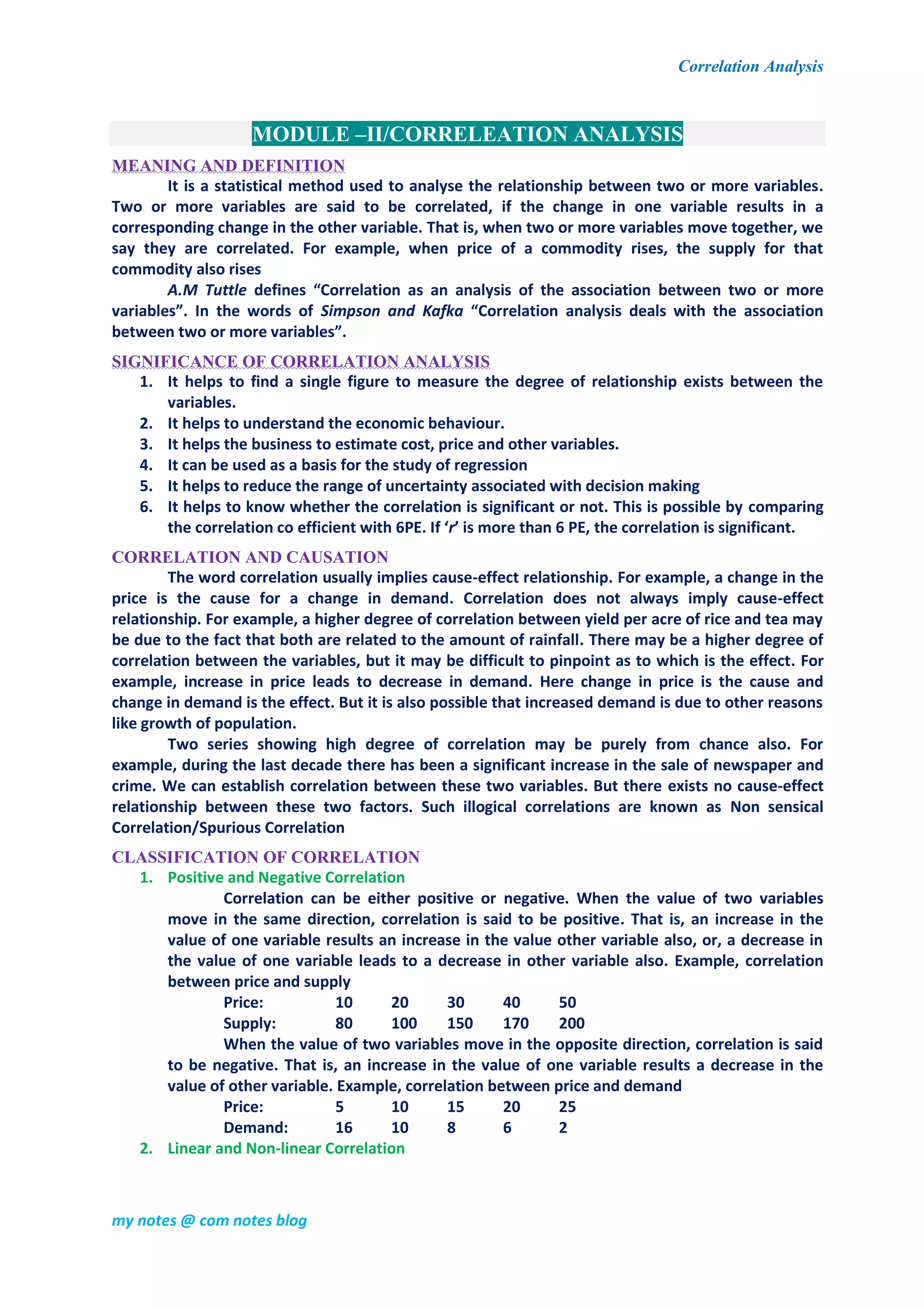
1. Positive and Negative Correlation
Correlation can be either positive or negative. When the value of two variables
move in the same direction, correlation is said to be positive. That is, an increase in the
value of one variable results an increase in the value other variable also, or, a decrease in
the value of one variable leads to a decrease in other variable also. Example, correlation
between price and supply
Price: 10 20 30 40 50
Supply: 80 100 150 170 200
When the value of two variables move in the opposite direction, correlation is said
to be negative. That is, an increase in the value of one variable results a decrease in the
value of other variable. Example, correlation between price and demand
Price: 5 10 15 20 25
Demand: 16 10 8 6 2
2. Linear and Non-linear Correlation
Correlation Analysis
my notes @ com notes blog
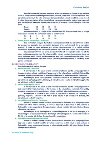
Correlation may be linear or nonlinear. When the amount of change in one variable
leads to a constant ratio of change in the other variable, correlation is said to be linear. In a
correlation analysis, if the ratio of change between the two sets of variable is same, then it
is called linear correlation. When there is linear correlation, the point plotted on a graph will
give a straight line. Example, if price goes up by 10%, it leads to a rise in supply by 15% each
time
Price: 10 15 30 60
Supply: 50 75 150 300
When the amount of change in one variable does not bring the same ratio of change
in the other variable, the correlation is said to be non-linear
X: 2 4 6 10 15
Y: 8 10 18 22 26
3. Simple, Partial and Multiple Correlation
In a correlation analysis, if only two variables are studied, the correlation is said to
be simple. For example, the correlation between price and demand. In a correlation
analysis, if three or more variables are studied simultaneously, it is called multiple
correlations. For example, the correlation between yield with both rainfall and temperature
In partial correlation, we study the relationship of one variable with one of the
other variables presuming that the other variables remain constant. For example, there are
three variables- yield, rainfall and temperature. And each is related with the other. Then,
the relationship between yield and rainfall (assuming the temperature is constant) is the
partial correlation
DEGREES OF CORRELATION
Correlation exists in various degrees
1. Perfect Positive Correlation
If an increase in the value of one variable is followed by the same proportion of
increase in other related variable or if a decrease in the value of one variable is followed by
the same proportion of decrease in other related variable, it is perfect positive correlation.
For example, if 10% rise in price of a commodity results in 10% rise in its supply, the
correlation is perfectly positive. Similarly, if 5% full in price results in 5% fall in supply, the
correlation is perfectly positive.
2. Perfect Negative Correlation
If an increase in the value of one variable is followed by the same proportion of
decrease in other related variable or if a decrease in the value of one variable is followed by
the same proportion of increase in other related variably it is Perfect Negative Correlation.
For example, if 10% rise in price results in 10% fall in its demand the correlation is
perfectly negative. Similarly if 5% fall in price results in 5% increase in demand, the
correlation is perfectly negative.
3. Limited Degree of Positive Correlation
When an increase in the value of one variable is followed by a non-proportional
increase in other related variable, or when a decrease in the value of one variable is
followed by a non-proportional decrease in other related variable, it is called limited degree
of positive correlation.
For example, if 10% rise in price of a commodity results in 5% rise in its supply, it is
limited degree of positive correlation. Similarly if 10% fall in price of a commodity results in
5% fall in its supply, it is limited degree of positive correlation.
4. Limited Degree of Negative Correlation
When an increase in the value of one variable is followed by a non-proportional
decrease in other related variable, or when a decrease in the value of one variable is
followed by a non-proportional increase in other related variable, it is called limited degree
of negative correlation.
Correlation Analysis
my notes @ com notes blog
For example, if 10% rise in price results in 5% fall in its demand, it is limited degree
of negative correlation. Similarly, if 5% fall in price results in 10% increase in demand, it is
limited degree of negative correlation.
5. Zero Correlation/Zero Degree Correlation
If there is no correlation between variables it is called zero correlation. In other
words, if the values of one variable cannot be associated with the values of the other
variable, it is zero correlation.
METHODS OF STUDYING CORRELATION
1. Graphic method
a) Scatter diagram
b) Correlation graph
2. Algebraic methods/Mathematical methods/statistical methods/Co-efficient of correlation
methods
a) Karl Pearson’s Co-efficient of correlation
b) Spear man’s Rank correlation method
c) Concurrent deviation method
SCATTER DIAGRAM
It is also known as dot chart. It is a graphical method of studying correlation between two
variables. It is a visual aid to show the presence or absence of correlation between two variables.
In scatter diagram, one of the variables is shown on the X-axis and the other on Y-axis. Each
pair of values is plotted by means of a dot mark. If these dot marks show some trends either
upward or downward, the two variables are said to be correlated. If the plotted dots do not show
any trend, the two variables are not correlated. The greater the scatter of the dots, the lower is the
relationship
Merits of Scatter Diagram Method
1. It is a simple method of studying correlation between variables.
2. It is a non-mathematical method of studying correlation between the variables
3. It is very easy to understand
4. It is not affected by the size of extreme values
5. Making a scatter diagram is, usually, the first step in investigating the relationship between
two variables.
Demerits of Scatter Diagram Method
1. It gives only a rough idea about the correlation between variables.
2. Further algebraic treatment is not possible. The numerical measurement of correlation co-
efficient cannot be made under this method.
3. The exact degree of correlation between the variables cannot be easily determined
4. If the number of pairs of variables is either very big or very small, the method is not easy
CORRELATION GRAPH METHOD
Under correlation graph method the individual values of the two variables are plotted on a
graph paper. Then dots relating to these variables are joined separately so as to get two curves. By
examining the direction and closeness of the two curves, we can infer whether the variables are
related or not. If both the curves are moving in the same direction (either upward or downward)
correlation is said to be positive. If the curves are moving in the opposite directions, correlation is
said to be negative.
Merits of Correlation Graph Method
1. This is a simple method of studying correlation between the variable
2. This does not require mathematical calculations.
3. This method is very easy to understand
Demerits of Correlation Graph Method:
Correlation Analysis
my notes @ com notes blog
1. A numerical value of correlation cannot be calculated.
2. It is only a pictorial presentation of the relationship between variables.
3. It is not possible to establish the exact degree of relationship between the variables.
MATHEMATICAL/STATISTICAL CORRELATION/CO-EFFICIENT OF CORRELATION
It is an algebraic method of measuring correlation. It shows the degree or extent of
correlation between two variables. It covers:
1. Karl Pearson’s co-efficient of correlation
2. Spearman’s rank correlation
3. Concurrent deviation
Karl Pearson’s Co-Efficient of Correlation or Pearsonian Co-Efficient of Correlation
It was developed by the reputed statistician and biologist Prof: Karl Pearson. It is denoted
by r. It is also known as product moment correlation co-efficient.
Assumptions
1. There is a possibility of linear relationship between variables.
2. The variables are affected by a large number of dependent causes so as to to form a normal
distribution.
3. There is a cause-effect relationship between the variables.
Properties
1. It has a well-defined formula.
2. It is a pure number and is independent of the units of measurement.
3. It lies in between ±1
4. It is the geometric mean of the two regressions co-efficient.
5. It does not change with reference to change of origin or change of scales.
6. Co-efficient of correlation between x and y is same as that between y and x
Methods
a) When deviations are taken from assumed mean
b) When deviations are taken from assumed mean
When deviations are taken from assumed mean
STEPS:
1. Take the deviations of x series from the mean of x which is denoted by x or dx
2. Square these deviations and get total. That is, Ʃx2
or Ʃdx2
.
3. Take the deviations of y series from the mean of y which is denoted by y or dy
4. Square these deviations and get total. That is, Ʃy2
or Ʃdy2
.
5. Multiply the deviations of x and y series, and get the total. That is Ʃdx.dy
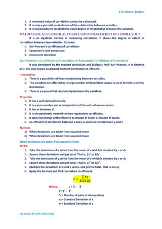
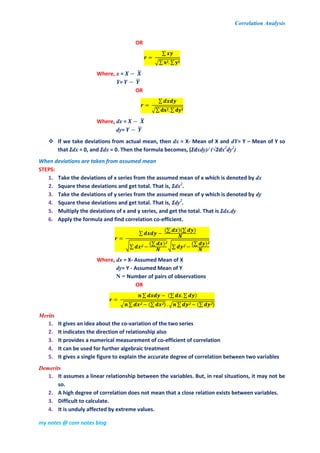
6. Apply the formula and find correlation co-efficient.
∑
Where, x = ̅
Y= ̅
N = Number of pairs of observations
σx= Standard Deviation of x
σy= Standard Deviation of y
Correlation Analysis
my notes @ com notes blog
OR
∑
√∑ ∑
Where, x = ̅
Y= ̅
OR
∑
√∑ ∑
Where, dx = ̅
dy= ̅
 If we take deviations from actual mean, then dx = X- Mean of X and dY= Y – Mean of Y so
that Ʃdx = 0, and Ʃdx = 0. Then the formula becomes, (Ʃdxdy)/ (√Ʃdx2
dy2
)
When deviations are taken from assumed mean
STEPS:
1. Take the deviations of x series from the assumed mean of x which is denoted by dx
2. Square these deviations and get total. That is, Ʃdx2
.
3. Take the deviations of y series from the assumed mean of y which is denoted by dy
4. Square these deviations and get total. That is, Ʃdy2
.
5. Multiply the deviations of x and y series, and get the total. That is Ʃdx.dy
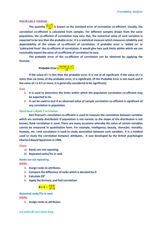
6. Apply the formula and find correlation co-efficient.
∑
(∑ )(∑ )
√∑
(∑ ) √∑
(∑ )
Where, dx = X- Assumed Mean of X
dy= Y - Assumed Mean of Y
N = Number of pairs of observations
OR
∑ (∑ ∑ )
√ ∑ (∑ ) √ ∑ (∑ )
Merits
1. It gives an idea about the co-variation of the two series
2. It indicates the direction of relationship also
3. It provides a numerical measurement of co-efficient of correlation
4. It can be used for further algebraic treatment
5. It gives a single figure to explain the accurate degree of correlation between two variables
Demerits
1. It assumes a linear relationship between the variables. But, in real situations, it may not be
so.
2. A high degree of correlation does not mean that a close relation exists between variables.
3. Difficult to calculate.
4. It is unduly affected by extreme values.
Correlation Analysis
my notes @ com notes blog
PROBABLE ERROR
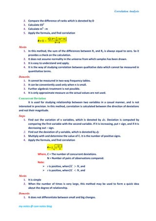
The quantity
( )
√
is known as the standard error of correlation co-efficient. Usually, the
correlation co-efficient is calculated from samples. For different samples drawn from the same
population, the co-efficient of correlation may vary. But, the numerical value of such variation is
expected to be less than the probable error. It is a statistical measure which measures reliability and
dependability of the values of co-efficient of correlation. If probable error is ‘added to’ or
‘subtracted from’ the co-efficient of correlation, it would give two such limits within which we can
reasonably expect the value of co-efficient of correlation to vary.
The probable error of the co-efficient of correlation can be obtained by applying the
formula:
Probable Error =
( )
√
If the value of r is less than the probable error, it is not at all significant. If the value of r is
more than six times of the probable error, it is significant. (If the Probable Error is not much and if
the value of r is 0.5 or more, it is generally considered to be significant)
Uses
1. It is used to determine the limits within which the population correlation co-efficient may
be expected to lie.
2. It can be used to test if an observed value of sample correlation co-efficient is significant of
any correlation in population.
Spearman’s Rank Correlation
Karl Pearson’s correlation co-efficient is used to measure the correlation between variables
which are normally distributed. If population is not normal, or the shape of the distribution is not
known, Rank correlation is used. There are many occasions whereby the value of certain variables
cannot be measured in quantitative form. For example, intelligence, beauty, character, morality,
honesty, etc. rank correlation is used to study association between such variables. It is a method
used to study the correlation between attributes. It was developed by the British psychologist
Charles Edward Spearman in 1904.
Cases
a) Ranks are not repeating
b) Repeated ranks/Tie in rank
Ranks are not repeating
STEPS:
1. Assign ranks to attributes
2. Compare the difference of ranks which is denoted by D
3. Calculate ƩD2
4. Apply the formula, and find correlation
R =
∑
Repeated ranks/Tie in rank
STEPS:
1. Assign ranks to attributes
Correlation Analysis
my notes @ com notes blog
2. Compare the difference of ranks which is denoted by D
3. Calculate ƩD2
4. Calculate m3
- m
5. Apply the formula, and find correlation
R =
⌊∑ ( )⌋
Merits
1. In this method, the sum of the differences between R1 and R2 is always equal to zero. So it
provides a check on the calculation.
2. It does not assume normality in the universe from which samples has been drawn.
3. It is easy to understand and apply.
4. It is the way of studying correlation between qualitative data which cannot be measured in
quantitative terms.
Demerits
1. It cannot be measured in two-way frequency tables.
2. It can be conveniently used only when n is small.
3. Further algebraic treatment is not possible.
4. It is only approximate measure as the actual values are not used.
Concurrent Deviation
It is used for studying relationship between two variables in a casual manner, and is not
interested in precision. In this method, correlation is calculated between the direction of deviations
and not their magnitude.
Steps
1. Find out the variation of x variables, which is denoted by dx. Deviation is computed by
comparing the first variable with the second variable. If it is increasing, put + sign, and if it is
decreasing out – sign.
2. Find out the deviation of y variable, which is denoted by dy
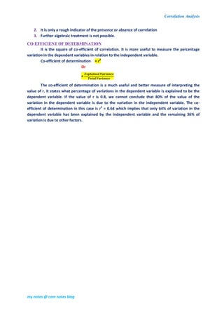
3. Multiply with and determine the value of C. it is the number of positive signs.
4. Apply the formula, and find correlation
R = √
Where, C = The number of concurrent deviations.
N = Number of pairs of observations compared.
Note:
 r is positive, when , and
Merits
1. It is simple
2. When the number of times is very large, this method may be used to form a quick idea
about the degree of relationship.
Demerits
1. It does not differentiate between small and big changes.
Correlation Analysis
my notes @ com notes blog
2. It is only a rough indicator of the presence or absence of correlation
3. Further algebraic treatment is not possible.
CO-EFFICIENT OF DETERMINATION
It is the square of co-efficient of correlation. It is more useful to measure the percentage
variation in the dependent variables in relation to the independent variable.
Co-efficient of determination = r2
Or
=
The co-efficient of determination is a much useful and better measure of interpreting the
value of r. it states what percentage of variations in the dependent variable is explained to be the
dependent variable. If the value of r is 0.8, we cannot conclude that 80% of the value of the
variation in the dependent variable is due to the variation in the independent variable. The co-
efficient of determination in this case is r2
= 0.64 which implies that only 64% of variation in the
dependent variable has been explained by the independent variable and the remaining 36% of
variation is due to other factors.

03 correlation analysis

  • 1.
    Correlation Analysis my notes@ com notes blog MODULE –II/CORRELEATION ANALYSIS MEANING AND DEFINITION It is a statistical method used to analyse the relationship between two or more variables. Two or more variables are said to be correlated, if the change in one variable results in a corresponding change in the other variable. That is, when two or more variables move together, we say they are correlated. For example, when price of a commodity rises, the supply for that commodity also rises A.M Tuttle defines “Correlation as an analysis of the association between two or more variables”. In the words of Simpson and Kafka “Correlation analysis deals with the association between two or more variables”. SIGNIFICANCE OF CORRELATION ANALYSIS 1. It helps to find a single figure to measure the degree of relationship exists between the variables. 2. It helps to understand the economic behaviour. 3. It helps the business to estimate cost, price and other variables. 4. It can be used as a basis for the study of regression 5. It helps to reduce the range of uncertainty associated with decision making 6. It helps to know whether the correlation is significant or not. This is possible by comparing the correlation co efficient with 6PE. If ‘r’ is more than 6 PE, the correlation is significant. CORRELATION AND CAUSATION The word correlation usually implies cause-effect relationship. For example, a change in the price is the cause for a change in demand. Correlation does not always imply cause-effect relationship. For example, a higher degree of correlation between yield per acre of rice and tea may be due to the fact that both are related to the amount of rainfall. There may be a higher degree of correlation between the variables, but it may be difficult to pinpoint as to which is the effect. For example, increase in price leads to decrease in demand. Here change in price is the cause and change in demand is the effect. But it is also possible that increased demand is due to other reasons like growth of population. Two series showing high degree of correlation may be purely from chance also. For example, during the last decade there has been a significant increase in the sale of newspaper and crime. We can establish correlation between these two variables. But there exists no cause-effect relationship between these two factors. Such illogical correlations are known as Non sensical Correlation/Spurious Correlation CLASSIFICATION OF CORRELATION 1. Positive and Negative Correlation Correlation can be either positive or negative. When the value of two variables move in the same direction, correlation is said to be positive. That is, an increase in the value of one variable results an increase in the value other variable also, or, a decrease in the value of one variable leads to a decrease in other variable also. Example, correlation between price and supply Price: 10 20 30 40 50 Supply: 80 100 150 170 200 When the value of two variables move in the opposite direction, correlation is said to be negative. That is, an increase in the value of one variable results a decrease in the value of other variable. Example, correlation between price and demand Price: 5 10 15 20 25 Demand: 16 10 8 6 2 2. Linear and Non-linear Correlation
  • 2.
    Correlation Analysis my notes@ com notes blog Correlation may be linear or nonlinear. When the amount of change in one variable leads to a constant ratio of change in the other variable, correlation is said to be linear. In a correlation analysis, if the ratio of change between the two sets of variable is same, then it is called linear correlation. When there is linear correlation, the point plotted on a graph will give a straight line. Example, if price goes up by 10%, it leads to a rise in supply by 15% each time Price: 10 15 30 60 Supply: 50 75 150 300 When the amount of change in one variable does not bring the same ratio of change in the other variable, the correlation is said to be non-linear X: 2 4 6 10 15 Y: 8 10 18 22 26 3. Simple, Partial and Multiple Correlation In a correlation analysis, if only two variables are studied, the correlation is said to be simple. For example, the correlation between price and demand. In a correlation analysis, if three or more variables are studied simultaneously, it is called multiple correlations. For example, the correlation between yield with both rainfall and temperature In partial correlation, we study the relationship of one variable with one of the other variables presuming that the other variables remain constant. For example, there are three variables- yield, rainfall and temperature. And each is related with the other. Then, the relationship between yield and rainfall (assuming the temperature is constant) is the partial correlation DEGREES OF CORRELATION Correlation exists in various degrees 1. Perfect Positive Correlation If an increase in the value of one variable is followed by the same proportion of increase in other related variable or if a decrease in the value of one variable is followed by the same proportion of decrease in other related variable, it is perfect positive correlation. For example, if 10% rise in price of a commodity results in 10% rise in its supply, the correlation is perfectly positive. Similarly, if 5% full in price results in 5% fall in supply, the correlation is perfectly positive. 2. Perfect Negative Correlation If an increase in the value of one variable is followed by the same proportion of decrease in other related variable or if a decrease in the value of one variable is followed by the same proportion of increase in other related variably it is Perfect Negative Correlation. For example, if 10% rise in price results in 10% fall in its demand the correlation is perfectly negative. Similarly if 5% fall in price results in 5% increase in demand, the correlation is perfectly negative. 3. Limited Degree of Positive Correlation When an increase in the value of one variable is followed by a non-proportional increase in other related variable, or when a decrease in the value of one variable is followed by a non-proportional decrease in other related variable, it is called limited degree of positive correlation. For example, if 10% rise in price of a commodity results in 5% rise in its supply, it is limited degree of positive correlation. Similarly if 10% fall in price of a commodity results in 5% fall in its supply, it is limited degree of positive correlation. 4. Limited Degree of Negative Correlation When an increase in the value of one variable is followed by a non-proportional decrease in other related variable, or when a decrease in the value of one variable is followed by a non-proportional increase in other related variable, it is called limited degree of negative correlation.
  • 3.
    Correlation Analysis my notes@ com notes blog For example, if 10% rise in price results in 5% fall in its demand, it is limited degree of negative correlation. Similarly, if 5% fall in price results in 10% increase in demand, it is limited degree of negative correlation. 5. Zero Correlation/Zero Degree Correlation If there is no correlation between variables it is called zero correlation. In other words, if the values of one variable cannot be associated with the values of the other variable, it is zero correlation. METHODS OF STUDYING CORRELATION 1. Graphic method a) Scatter diagram b) Correlation graph 2. Algebraic methods/Mathematical methods/statistical methods/Co-efficient of correlation methods a) Karl Pearson’s Co-efficient of correlation b) Spear man’s Rank correlation method c) Concurrent deviation method SCATTER DIAGRAM It is also known as dot chart. It is a graphical method of studying correlation between two variables. It is a visual aid to show the presence or absence of correlation between two variables. In scatter diagram, one of the variables is shown on the X-axis and the other on Y-axis. Each pair of values is plotted by means of a dot mark. If these dot marks show some trends either upward or downward, the two variables are said to be correlated. If the plotted dots do not show any trend, the two variables are not correlated. The greater the scatter of the dots, the lower is the relationship Merits of Scatter Diagram Method 1. It is a simple method of studying correlation between variables. 2. It is a non-mathematical method of studying correlation between the variables 3. It is very easy to understand 4. It is not affected by the size of extreme values 5. Making a scatter diagram is, usually, the first step in investigating the relationship between two variables. Demerits of Scatter Diagram Method 1. It gives only a rough idea about the correlation between variables. 2. Further algebraic treatment is not possible. The numerical measurement of correlation co- efficient cannot be made under this method. 3. The exact degree of correlation between the variables cannot be easily determined 4. If the number of pairs of variables is either very big or very small, the method is not easy CORRELATION GRAPH METHOD Under correlation graph method the individual values of the two variables are plotted on a graph paper. Then dots relating to these variables are joined separately so as to get two curves. By examining the direction and closeness of the two curves, we can infer whether the variables are related or not. If both the curves are moving in the same direction (either upward or downward) correlation is said to be positive. If the curves are moving in the opposite directions, correlation is said to be negative. Merits of Correlation Graph Method 1. This is a simple method of studying correlation between the variable 2. This does not require mathematical calculations. 3. This method is very easy to understand Demerits of Correlation Graph Method:
  • 4.
    Correlation Analysis my notes@ com notes blog 1. A numerical value of correlation cannot be calculated. 2. It is only a pictorial presentation of the relationship between variables. 3. It is not possible to establish the exact degree of relationship between the variables. MATHEMATICAL/STATISTICAL CORRELATION/CO-EFFICIENT OF CORRELATION It is an algebraic method of measuring correlation. It shows the degree or extent of correlation between two variables. It covers: 1. Karl Pearson’s co-efficient of correlation 2. Spearman’s rank correlation 3. Concurrent deviation Karl Pearson’s Co-Efficient of Correlation or Pearsonian Co-Efficient of Correlation It was developed by the reputed statistician and biologist Prof: Karl Pearson. It is denoted by r. It is also known as product moment correlation co-efficient. Assumptions 1. There is a possibility of linear relationship between variables. 2. The variables are affected by a large number of dependent causes so as to to form a normal distribution. 3. There is a cause-effect relationship between the variables. Properties 1. It has a well-defined formula. 2. It is a pure number and is independent of the units of measurement. 3. It lies in between ±1 4. It is the geometric mean of the two regressions co-efficient. 5. It does not change with reference to change of origin or change of scales. 6. Co-efficient of correlation between x and y is same as that between y and x Methods a) When deviations are taken from assumed mean b) When deviations are taken from assumed mean When deviations are taken from assumed mean STEPS: 1. Take the deviations of x series from the mean of x which is denoted by x or dx 2. Square these deviations and get total. That is, Ʃx2 or Ʃdx2 . 3. Take the deviations of y series from the mean of y which is denoted by y or dy 4. Square these deviations and get total. That is, Ʃy2 or Ʃdy2 . 5. Multiply the deviations of x and y series, and get the total. That is Ʃdx.dy 6. Apply the formula and find correlation co-efficient. ∑ Where, x = ̅ Y= ̅ N = Number of pairs of observations σx= Standard Deviation of x σy= Standard Deviation of y
  • 5.
    Correlation Analysis my notes@ com notes blog OR ∑ √∑ ∑ Where, x = ̅ Y= ̅ OR ∑ √∑ ∑ Where, dx = ̅ dy= ̅  If we take deviations from actual mean, then dx = X- Mean of X and dY= Y – Mean of Y so that Ʃdx = 0, and Ʃdx = 0. Then the formula becomes, (Ʃdxdy)/ (√Ʃdx2 dy2 ) When deviations are taken from assumed mean STEPS: 1. Take the deviations of x series from the assumed mean of x which is denoted by dx 2. Square these deviations and get total. That is, Ʃdx2 . 3. Take the deviations of y series from the assumed mean of y which is denoted by dy 4. Square these deviations and get total. That is, Ʃdy2 . 5. Multiply the deviations of x and y series, and get the total. That is Ʃdx.dy 6. Apply the formula and find correlation co-efficient. ∑ (∑ )(∑ ) √∑ (∑ ) √∑ (∑ ) Where, dx = X- Assumed Mean of X dy= Y - Assumed Mean of Y N = Number of pairs of observations OR ∑ (∑ ∑ ) √ ∑ (∑ ) √ ∑ (∑ ) Merits 1. It gives an idea about the co-variation of the two series 2. It indicates the direction of relationship also 3. It provides a numerical measurement of co-efficient of correlation 4. It can be used for further algebraic treatment 5. It gives a single figure to explain the accurate degree of correlation between two variables Demerits 1. It assumes a linear relationship between the variables. But, in real situations, it may not be so. 2. A high degree of correlation does not mean that a close relation exists between variables. 3. Difficult to calculate. 4. It is unduly affected by extreme values.
  • 6.
    Correlation Analysis my notes@ com notes blog PROBABLE ERROR The quantity ( ) √ is known as the standard error of correlation co-efficient. Usually, the correlation co-efficient is calculated from samples. For different samples drawn from the same population, the co-efficient of correlation may vary. But, the numerical value of such variation is expected to be less than the probable error. It is a statistical measure which measures reliability and dependability of the values of co-efficient of correlation. If probable error is ‘added to’ or ‘subtracted from’ the co-efficient of correlation, it would give two such limits within which we can reasonably expect the value of co-efficient of correlation to vary. The probable error of the co-efficient of correlation can be obtained by applying the formula: Probable Error = ( ) √ If the value of r is less than the probable error, it is not at all significant. If the value of r is more than six times of the probable error, it is significant. (If the Probable Error is not much and if the value of r is 0.5 or more, it is generally considered to be significant) Uses 1. It is used to determine the limits within which the population correlation co-efficient may be expected to lie. 2. It can be used to test if an observed value of sample correlation co-efficient is significant of any correlation in population. Spearman’s Rank Correlation Karl Pearson’s correlation co-efficient is used to measure the correlation between variables which are normally distributed. If population is not normal, or the shape of the distribution is not known, Rank correlation is used. There are many occasions whereby the value of certain variables cannot be measured in quantitative form. For example, intelligence, beauty, character, morality, honesty, etc. rank correlation is used to study association between such variables. It is a method used to study the correlation between attributes. It was developed by the British psychologist Charles Edward Spearman in 1904. Cases a) Ranks are not repeating b) Repeated ranks/Tie in rank Ranks are not repeating STEPS: 1. Assign ranks to attributes 2. Compare the difference of ranks which is denoted by D 3. Calculate ƩD2 4. Apply the formula, and find correlation R = ∑ Repeated ranks/Tie in rank STEPS: 1. Assign ranks to attributes
  • 7.
    Correlation Analysis my notes@ com notes blog 2. Compare the difference of ranks which is denoted by D 3. Calculate ƩD2 4. Calculate m3 - m 5. Apply the formula, and find correlation R = ⌊∑ ( )⌋ Merits 1. In this method, the sum of the differences between R1 and R2 is always equal to zero. So it provides a check on the calculation. 2. It does not assume normality in the universe from which samples has been drawn. 3. It is easy to understand and apply. 4. It is the way of studying correlation between qualitative data which cannot be measured in quantitative terms. Demerits 1. It cannot be measured in two-way frequency tables. 2. It can be conveniently used only when n is small. 3. Further algebraic treatment is not possible. 4. It is only approximate measure as the actual values are not used. Concurrent Deviation It is used for studying relationship between two variables in a casual manner, and is not interested in precision. In this method, correlation is calculated between the direction of deviations and not their magnitude. Steps 1. Find out the variation of x variables, which is denoted by dx. Deviation is computed by comparing the first variable with the second variable. If it is increasing, put + sign, and if it is decreasing out – sign. 2. Find out the deviation of y variable, which is denoted by dy 3. Multiply with and determine the value of C. it is the number of positive signs. 4. Apply the formula, and find correlation R = √ Where, C = The number of concurrent deviations. N = Number of pairs of observations compared. Note:  r is positive, when , and  r is positive, when , and Merits 1. It is simple 2. When the number of times is very large, this method may be used to form a quick idea about the degree of relationship. Demerits 1. It does not differentiate between small and big changes.
  • 8.
    Correlation Analysis my notes@ com notes blog 2. It is only a rough indicator of the presence or absence of correlation 3. Further algebraic treatment is not possible. CO-EFFICIENT OF DETERMINATION It is the square of co-efficient of correlation. It is more useful to measure the percentage variation in the dependent variables in relation to the independent variable. Co-efficient of determination = r2 Or = The co-efficient of determination is a much useful and better measure of interpreting the value of r. it states what percentage of variations in the dependent variable is explained to be the dependent variable. If the value of r is 0.8, we cannot conclude that 80% of the value of the variation in the dependent variable is due to the variation in the independent variable. The co- efficient of determination in this case is r2 = 0.64 which implies that only 64% of variation in the dependent variable has been explained by the independent variable and the remaining 36% of variation is due to other factors.