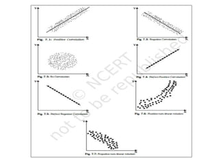
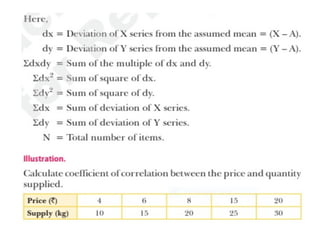
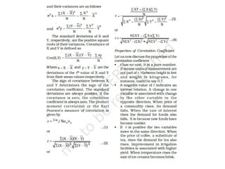
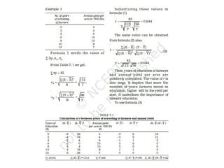
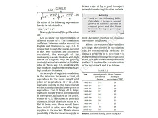
KARL PEARSON’S
CORRELATION METHOD
TASAWWUR HUSAIN ZAIDI
DEPARTMENT OF GEOGRAPHY
JAMIA MILLIA ISLAMIA
NEW DELHI 110025
HISTORY:
The concept of correlation originated in the 1880s with the works of Galton, F.. In
1888, in an article sent to the Royal Statistical Society entitled “Co-relations and their
measurement chiefly from anthropometric data,” Galton used the term “correlation”
for the first time, although he was still alternating between the terms “co-relation” and
“correlation” and he spoke of a “co-relation index.” On the other hand, he invoke the
concept of a negative correlation. According to Stigler (1989),Galton only appeared to
suggest that correlation was a positive relationship.
Pearson, Karl wrote in 1920 that correlation had been discovered by Galton, whose
work “Natural inheritance” (1889) pushed him to study this concept too, along with
two other researchers, Weldon and Edgeworth. Pearson and Edgeworth then
developed the theory of correlation.
Weldon thought the correlation coefficient should be called the “Galton function.”
However, Edgeworth replaced Galton’s term “correlation index” and Weldon’s term
“Galton function” by the term “correlation coefficient.”
According to Mudholkar (1982), Pearson, K. systemized the analysis of correlation and
established a theory of correlation for three variables. Researchers from University
College, most notably his assistant Yule, G.U., were also interested in developing
multiple correlation. Spearman published the first study on rank correlation in 1904.
Among the works that were carried out in this field, it is worth highlighting those of
Yule, who in an article entitled “Why do we sometimes get non-sense-correlation
between time-series” (1926) discussed the problem of correlation analysis
interpretation. Finally, correlation robustness was investigated by Mosteller and Tukey
(1977).
MEANING AND DEFINITION OF CORRELATION
If the changes in the values of one variable are accompanied by changes in the values of
the other variable, then the variables are said to be correlated. Correlation studies and
measures the direction and intensity of relationship among variables. Correlation
measures covariation, not causation. Correlation should never be interpreted as
implying cause and effect relation.
According to Croxton and Cowden, “When the relationship is of a quantitative
nature, the appropriate statistical tool for discovering and measuring the relationship
and expressing it in a brief formula is known as correlation”.
In the words of Boddington, “Whenever some define connection exists between the
two or more groups, classes or series or data there is said lo be correlation”.
The presence of correlation between two variables X and Y simply means that when the
value of one variable is found to change in one direction, the value of the other variable
is found to change either in the same direction (i.e. positive change) or in the opposite
direction (i.e. negative change), but in a definite way. For simplicity we assume here
that the correlation, if it exists, is linear, i.e. the relative movement of the two variables
can be represented by drawing a straight line on graph paper.
TYPES OF RELATIONSHIP
•Cause and Effect Relationship (rainfall and crop productivity, Income and
expenditure)
•Coincidence (arrival of migratory birds in a sanctuary and the birth rates in the
locality)
•Third Variable’s Impact (Brisk sale of ice-creams may be related to higher number of
deaths due to drowning)
Correlation does not imply causality.
Height and vocabulary of children are correlated – both increase with age. Clearly, an
increase in height does not cause an increase in vocabulary, or vice versa. Other
examples are less clear. Years of education and income are known to be correlated.
Nevertheless, one cannot deduce that more education causes higher income.
Correlations may be weak or strong, positive or negative, and linear or nonlinear.
TYPES OF CORRELATION
POSITIVE AND NEGATIVE CORRELATION
(1) Positive Correlation: When two variables move in the same direction, that is, when one
increases the other also increases and when one decreases the other also decreases, such a relation
is called positive correlation.
(2) Negative Correlation: When two variables change in different directions, itis called negative
correlation. Relationship between price and demand, may be cited as an example.
LINEAR AND NON-LINEAR CORRELATION
(1) Linear Correlation: When two variables change in a constant proportion, it is called linear
correlation. If the two sets of data bearing fixed proportion to each other are shown on a graph
paper, their relationship will be indicated by a straight line. Thus, linear correlation implies a
straight line relationship.
(2) Non-linear Correlation: When the two variables do not change in any constant proportion,
the relationship is said to be non-linear. Such a relationship does not form a straight line
relationship.
SIMPLE AND MULTIPLE CORRELATION
(1) Simple Correlation: implies the study of relationship between two variables only. Like the
relationship between price and demand or the relationship between money supply and price level.
(2) Multiple Correlation: When the relationship among three or more than three variables is
studied simultaneously, it is called multiple correlation. In case of such correlation, the entire set of
independent and dependent variables is simultaneously studied. For instance, effects of rainfall,
manure, water, etc., on per hectare productivity of wheat are simultaneously studied.
DEGREE OF CORRELATION:
Degree of correlation refers to the Coefficient of Correlation. There can be the following degrees
of positive and negative correlation.
1. Perfect Correlation: When two variables change in the same proportion it is called perfect
correlation. It may be of two kinds:
(i) Perfect Positive: Correlation is perfectly positive when proportional change in two variables
is in the same direction. In this case, coefficient of correlation is positive (+1).
(ii) Perfect Negative: Correlation is perfectly negative when proportional change in two
variables is in the opposite direction. In this case, coefficient of correlation is negative (-1).
2. Absence of Correlation: If there is no relation between two series or variables, that is, change
in one has no effect on the change in other, then those series or variables lack any correlation
between them.
3. Limited Degree of Correlation: Between perfect correlation and absence of correlation there
is a situation of limited degree of correlation. In real life, one mostly finds limited degree of
correlation. Its coefficient (r) is more than zero and less than one (r > 0 but < 1). The degree of
correlation between 0 and | may be rated as:
(i) High: When correlation of two series is close to one, it is called high degree of correlation. Its
coefficient lies between 0.75 and 1.
(ii) Moderate: When correlation of two series is neither large nor small, it is called moderate
degree of correlation. Its coefficient lies between 0.25 and 0.75.
(iii) Low: When the degree of correlation of two series is very small, it is called low degree of
correlation. Its coefficient lies between 0 and 0.25.
KARL PEARSON’S COEFFICIENT OF CORRELATION
This is also known as product moment correlation coefficient or simple correlation
coefficient. It gives a precise numerical value of the degree of linear relationship between two
variables X and Y.
It is important to note that Karl Pearson’s coefficient of correlation should be used only when
there is a linear relation between the variables. When there is a non-linear relation between X
and Y, then calculating the Karl Pearson’s coefficient of correlation can be misleading. Thus, if
the true relation is of the linear type as shown by the scatter diagrams in figures 7.1, 7.2, 7.4
and 7.5, then the Karl Pearson’s coefficient of correlation should be calculated and it will tell
us the direction and intensity of the relation between the variables. But if the true relation is of
the type shown in the scatter diagrams in Figures 7.6 or 7.7, then it means there is a non-linear
relation between X and Y and we should not try to use the Karl Pearson’s coefficient of
correlation.
It is, therefore, advisable to first examine the scatter diagram of the relation between the
variables before calculating the Karl Pearson’s correlation coefficient.
Let X1, X2, ..., XN be N values of X and Y1, Y2 ,..., YN be the corresponding values of Y. In
the subsequent presentations, the subscripts indicating the unit are dropped for the sake of
simplicity. The arithmetic means of X and Y are defined as
METHODS OF ESTIMATING CORRELATION
Various methods are available for estimating correlation between different sets of
statistical series. Some of the important ones are as under:
(1) Scattered Diagram Method,
(2) Karl Pearson's Coefficient of Correlation, and
(3) Spearman’s Rank Correlation Coefficient.
Scattered Diagram
Scattered diagram offers a graphic expression of the direction and degree of
correlation. To make a Scattered Diagram, data are plotted on a graph paper. A dot is
marked for each value. The course of these dots would indicate direction and
closeness of the variables. Following pictures show some of the possible directions
and the
degrees of closeness of the variables.
As should be clear from the scattered diagrams, closeness of the dots towards each
other in a particular direction indicates higher degree of correlation. If the dots are
scattered (showing neither the closeness nor any direction), it is an indication of low
degree of correlation.
MERITS AND DEMERITS OF SCATTERED DIAGRAM
Merits
(i) Scattered diagram is a very simple method of studying correlation between two
variables.
(ii) Just a glance at the diagram is enough to know if the values of the variables have
any relation or not.
(iii) Scattered diagram also indicates whether the relation is posilive or negative.
Demerits
(i) A scattered diagram does not measure the precise extent of correlation.
(ii) It gives only an approximate idea of the relationship.
(iii) Itis nota quantitative measure of the relationship between the variables. It is only a
qualitative expression of the quantitative change.
KARL PEARSON'S COEFFICIENT OF CORRELATION
Scattered diagram method of correlation merely indicates the direction of correlation
but not its precise magnitude. Karl Pearson has given a quantitative method of
calculating correlation. It is an important and widely used method of studying
correlation. Karl Pearsons’ coefficient of correlation is generally written as ‘r’.
FORMULA
According to Karl Pearson's method, the coefficient of correlation is measured as:
This formula is applied only to those series where deviations are worked out from actual
average of the series, it does not apply to those series where deviations are calculated on
the basis of assumed mean. Value of the coefficient of correlation calculated on the
basis of this formula may vary between +1 and -1. However, the situations, when r = +1,
r = 0, are rather rare. Generally, value of ‘r’ varies between +1 and -1.
A Modified Version of Karl Pearson's Formula
In it there is no need to calculate standard deviation of *X’ and ‘Y’. Coefficient of
correlation may be worked out directly using the following formula:
Short-cut Method
This method is used when mean value is not in whole number but in fractions. In this
method, deviation is calculated by taking the assumed mean of both the series. It
involves the following steps:
(i) Any convenient value in X and Y series is taken as assumed mean AX and AY.
(ii) With the help of assumed mean of both the series, deviation of the values of
individual variable, i.e., dx (X - AX) and dy (Y - AY) are calculated.
(iii) Σdx and Σdy are found by adding the deviations.
(iv) Deviations of the two series are multiplied, as dx.dy, and the multiples added up to
obtain Σdxdy.
(v) Squares of the deviations dx2
and dy2
are added up to find out Σdx2
and Σdy2
.
(vi) Finally, coefficient of correlation is calculated using the following formula:
CALCULATE PEARSON’S CORRELATION COEFFICIENT
1.In the SPSS menu, go to Analyze > Correlate > Bivariate.
2.In the Bivariate Correlations dialog box:
1. Select both Hours and Score from the variable list on the left and move
them to the Variables box on the right.
2. Ensure Pearson is checked under Correlation Coefficients (this is selected
by default).
3. Check Two-tailed under Test of Significance if you want a two-tailed
significance test. This option is commonly used unless you have a specific
reason to use a one-tailed test.
4. Optionally, check Flag significant correlations to indicate statistically
significant correlations in the output.
3.Click OK to run the correlation analysis.
ONE TIALED AND TWO TAILED TEST
Two-tailed test
One-tailed and two-tailed tests are statistical hypothesis tests that differ in how they
specify the direction of a potential relationship between variables:
•One-tailed test
Also known as a directional hypothesis, this test is used when the alternative hypothesis
specifies a direction. For example, a one-tailed test might be used to determine if a mean
is significantly greater than a given value, but not if it is significantly less.
Also known as a non-directional hypothesis, this test is used when the alternative
hypothesis does not specify a direction. For example, a two-tailed test might be used to
determine if a mean is significantly greater than or less than a given value.
Here are some things to keep in mind when using one-tailed and two-tailed tests:
•When to use a one-tailed test
A one-tailed test is appropriate when you have a strong reason to suspect that one version
is better than another. However, it's important to note that a one-tailed test only measures
the hypothesis in one direction, so it won't detect the opposite effect.
•When to use a two-tailed test
A two-tailed test is appropriate when you want to detect any difference, positive or
negative. It's also a good choice when you don't know the direction of the effect.
•When to state a one-tailed test
It's important to state the rationale for a one-tailed test before you start collecting data.
PROPERTIES OF CORRELATION COEFFICIENT
(i) r has no unit. It is a pure number. It means units of measurement are not parts of r.
(ii) A negative value of r indicates an inverse relation, and if r is positive, the two
variables move in the same direction.
(iii) If r = 0, the two variables are uncorrelated. There is no linear relation between
them. However, other types of relation may be there.
(iv) I fr = 1 or r = - 1, the correlation is perfect or proportionate. A high value of r
indicates strong linear relationship, i.e., + 1 or -l.
(v) The value of the correlation coefficient lies between minus one and plus one, i.e., -1
≤ r ≤ + 1. If the value of r lies outside this range, it indicates error in calculation.
KARL PEARSON’S CORRELATION METHOD (1).pptx

KARL PEARSON’S CORRELATION METHOD (1).pptx

  • 1.
    KARL PEARSON’S CORRELATION METHOD TASAWWURHUSAIN ZAIDI DEPARTMENT OF GEOGRAPHY JAMIA MILLIA ISLAMIA NEW DELHI 110025
  • 2.
    HISTORY: The concept ofcorrelation originated in the 1880s with the works of Galton, F.. In 1888, in an article sent to the Royal Statistical Society entitled “Co-relations and their measurement chiefly from anthropometric data,” Galton used the term “correlation” for the first time, although he was still alternating between the terms “co-relation” and “correlation” and he spoke of a “co-relation index.” On the other hand, he invoke the concept of a negative correlation. According to Stigler (1989),Galton only appeared to suggest that correlation was a positive relationship. Pearson, Karl wrote in 1920 that correlation had been discovered by Galton, whose work “Natural inheritance” (1889) pushed him to study this concept too, along with two other researchers, Weldon and Edgeworth. Pearson and Edgeworth then developed the theory of correlation. Weldon thought the correlation coefficient should be called the “Galton function.” However, Edgeworth replaced Galton’s term “correlation index” and Weldon’s term “Galton function” by the term “correlation coefficient.” According to Mudholkar (1982), Pearson, K. systemized the analysis of correlation and established a theory of correlation for three variables. Researchers from University College, most notably his assistant Yule, G.U., were also interested in developing multiple correlation. Spearman published the first study on rank correlation in 1904. Among the works that were carried out in this field, it is worth highlighting those of Yule, who in an article entitled “Why do we sometimes get non-sense-correlation between time-series” (1926) discussed the problem of correlation analysis interpretation. Finally, correlation robustness was investigated by Mosteller and Tukey (1977).
  • 3.
    MEANING AND DEFINITIONOF CORRELATION If the changes in the values of one variable are accompanied by changes in the values of the other variable, then the variables are said to be correlated. Correlation studies and measures the direction and intensity of relationship among variables. Correlation measures covariation, not causation. Correlation should never be interpreted as implying cause and effect relation. According to Croxton and Cowden, “When the relationship is of a quantitative nature, the appropriate statistical tool for discovering and measuring the relationship and expressing it in a brief formula is known as correlation”. In the words of Boddington, “Whenever some define connection exists between the two or more groups, classes or series or data there is said lo be correlation”. The presence of correlation between two variables X and Y simply means that when the value of one variable is found to change in one direction, the value of the other variable is found to change either in the same direction (i.e. positive change) or in the opposite direction (i.e. negative change), but in a definite way. For simplicity we assume here that the correlation, if it exists, is linear, i.e. the relative movement of the two variables can be represented by drawing a straight line on graph paper.
  • 4.
    TYPES OF RELATIONSHIP •Causeand Effect Relationship (rainfall and crop productivity, Income and expenditure) •Coincidence (arrival of migratory birds in a sanctuary and the birth rates in the locality) •Third Variable’s Impact (Brisk sale of ice-creams may be related to higher number of deaths due to drowning) Correlation does not imply causality. Height and vocabulary of children are correlated – both increase with age. Clearly, an increase in height does not cause an increase in vocabulary, or vice versa. Other examples are less clear. Years of education and income are known to be correlated. Nevertheless, one cannot deduce that more education causes higher income. Correlations may be weak or strong, positive or negative, and linear or nonlinear.
  • 5.
    TYPES OF CORRELATION POSITIVEAND NEGATIVE CORRELATION (1) Positive Correlation: When two variables move in the same direction, that is, when one increases the other also increases and when one decreases the other also decreases, such a relation is called positive correlation. (2) Negative Correlation: When two variables change in different directions, itis called negative correlation. Relationship between price and demand, may be cited as an example. LINEAR AND NON-LINEAR CORRELATION (1) Linear Correlation: When two variables change in a constant proportion, it is called linear correlation. If the two sets of data bearing fixed proportion to each other are shown on a graph paper, their relationship will be indicated by a straight line. Thus, linear correlation implies a straight line relationship. (2) Non-linear Correlation: When the two variables do not change in any constant proportion, the relationship is said to be non-linear. Such a relationship does not form a straight line relationship. SIMPLE AND MULTIPLE CORRELATION (1) Simple Correlation: implies the study of relationship between two variables only. Like the relationship between price and demand or the relationship between money supply and price level. (2) Multiple Correlation: When the relationship among three or more than three variables is studied simultaneously, it is called multiple correlation. In case of such correlation, the entire set of independent and dependent variables is simultaneously studied. For instance, effects of rainfall, manure, water, etc., on per hectare productivity of wheat are simultaneously studied.
  • 6.
    DEGREE OF CORRELATION: Degreeof correlation refers to the Coefficient of Correlation. There can be the following degrees of positive and negative correlation. 1. Perfect Correlation: When two variables change in the same proportion it is called perfect correlation. It may be of two kinds: (i) Perfect Positive: Correlation is perfectly positive when proportional change in two variables is in the same direction. In this case, coefficient of correlation is positive (+1). (ii) Perfect Negative: Correlation is perfectly negative when proportional change in two variables is in the opposite direction. In this case, coefficient of correlation is negative (-1). 2. Absence of Correlation: If there is no relation between two series or variables, that is, change in one has no effect on the change in other, then those series or variables lack any correlation between them. 3. Limited Degree of Correlation: Between perfect correlation and absence of correlation there is a situation of limited degree of correlation. In real life, one mostly finds limited degree of correlation. Its coefficient (r) is more than zero and less than one (r > 0 but < 1). The degree of correlation between 0 and | may be rated as: (i) High: When correlation of two series is close to one, it is called high degree of correlation. Its coefficient lies between 0.75 and 1. (ii) Moderate: When correlation of two series is neither large nor small, it is called moderate degree of correlation. Its coefficient lies between 0.25 and 0.75. (iii) Low: When the degree of correlation of two series is very small, it is called low degree of correlation. Its coefficient lies between 0 and 0.25.
  • 8.
    KARL PEARSON’S COEFFICIENTOF CORRELATION This is also known as product moment correlation coefficient or simple correlation coefficient. It gives a precise numerical value of the degree of linear relationship between two variables X and Y. It is important to note that Karl Pearson’s coefficient of correlation should be used only when there is a linear relation between the variables. When there is a non-linear relation between X and Y, then calculating the Karl Pearson’s coefficient of correlation can be misleading. Thus, if the true relation is of the linear type as shown by the scatter diagrams in figures 7.1, 7.2, 7.4 and 7.5, then the Karl Pearson’s coefficient of correlation should be calculated and it will tell us the direction and intensity of the relation between the variables. But if the true relation is of the type shown in the scatter diagrams in Figures 7.6 or 7.7, then it means there is a non-linear relation between X and Y and we should not try to use the Karl Pearson’s coefficient of correlation. It is, therefore, advisable to first examine the scatter diagram of the relation between the variables before calculating the Karl Pearson’s correlation coefficient. Let X1, X2, ..., XN be N values of X and Y1, Y2 ,..., YN be the corresponding values of Y. In the subsequent presentations, the subscripts indicating the unit are dropped for the sake of simplicity. The arithmetic means of X and Y are defined as
  • 9.
    METHODS OF ESTIMATINGCORRELATION Various methods are available for estimating correlation between different sets of statistical series. Some of the important ones are as under: (1) Scattered Diagram Method, (2) Karl Pearson's Coefficient of Correlation, and (3) Spearman’s Rank Correlation Coefficient. Scattered Diagram Scattered diagram offers a graphic expression of the direction and degree of correlation. To make a Scattered Diagram, data are plotted on a graph paper. A dot is marked for each value. The course of these dots would indicate direction and closeness of the variables. Following pictures show some of the possible directions and the degrees of closeness of the variables. As should be clear from the scattered diagrams, closeness of the dots towards each other in a particular direction indicates higher degree of correlation. If the dots are scattered (showing neither the closeness nor any direction), it is an indication of low degree of correlation.
  • 12.
    MERITS AND DEMERITSOF SCATTERED DIAGRAM Merits (i) Scattered diagram is a very simple method of studying correlation between two variables. (ii) Just a glance at the diagram is enough to know if the values of the variables have any relation or not. (iii) Scattered diagram also indicates whether the relation is posilive or negative. Demerits (i) A scattered diagram does not measure the precise extent of correlation. (ii) It gives only an approximate idea of the relationship. (iii) Itis nota quantitative measure of the relationship between the variables. It is only a qualitative expression of the quantitative change.
  • 13.
    KARL PEARSON'S COEFFICIENTOF CORRELATION Scattered diagram method of correlation merely indicates the direction of correlation but not its precise magnitude. Karl Pearson has given a quantitative method of calculating correlation. It is an important and widely used method of studying correlation. Karl Pearsons’ coefficient of correlation is generally written as ‘r’. FORMULA According to Karl Pearson's method, the coefficient of correlation is measured as: This formula is applied only to those series where deviations are worked out from actual average of the series, it does not apply to those series where deviations are calculated on the basis of assumed mean. Value of the coefficient of correlation calculated on the basis of this formula may vary between +1 and -1. However, the situations, when r = +1, r = 0, are rather rare. Generally, value of ‘r’ varies between +1 and -1.
  • 14.
    A Modified Versionof Karl Pearson's Formula In it there is no need to calculate standard deviation of *X’ and ‘Y’. Coefficient of correlation may be worked out directly using the following formula:
  • 16.
    Short-cut Method This methodis used when mean value is not in whole number but in fractions. In this method, deviation is calculated by taking the assumed mean of both the series. It involves the following steps: (i) Any convenient value in X and Y series is taken as assumed mean AX and AY. (ii) With the help of assumed mean of both the series, deviation of the values of individual variable, i.e., dx (X - AX) and dy (Y - AY) are calculated. (iii) Σdx and Σdy are found by adding the deviations. (iv) Deviations of the two series are multiplied, as dx.dy, and the multiples added up to obtain Σdxdy. (v) Squares of the deviations dx2 and dy2 are added up to find out Σdx2 and Σdy2 . (vi) Finally, coefficient of correlation is calculated using the following formula:
  • 21.
    CALCULATE PEARSON’S CORRELATIONCOEFFICIENT 1.In the SPSS menu, go to Analyze > Correlate > Bivariate. 2.In the Bivariate Correlations dialog box: 1. Select both Hours and Score from the variable list on the left and move them to the Variables box on the right. 2. Ensure Pearson is checked under Correlation Coefficients (this is selected by default). 3. Check Two-tailed under Test of Significance if you want a two-tailed significance test. This option is commonly used unless you have a specific reason to use a one-tailed test. 4. Optionally, check Flag significant correlations to indicate statistically significant correlations in the output. 3.Click OK to run the correlation analysis.
  • 22.
    ONE TIALED ANDTWO TAILED TEST Two-tailed test One-tailed and two-tailed tests are statistical hypothesis tests that differ in how they specify the direction of a potential relationship between variables: •One-tailed test Also known as a directional hypothesis, this test is used when the alternative hypothesis specifies a direction. For example, a one-tailed test might be used to determine if a mean is significantly greater than a given value, but not if it is significantly less. Also known as a non-directional hypothesis, this test is used when the alternative hypothesis does not specify a direction. For example, a two-tailed test might be used to determine if a mean is significantly greater than or less than a given value. Here are some things to keep in mind when using one-tailed and two-tailed tests: •When to use a one-tailed test A one-tailed test is appropriate when you have a strong reason to suspect that one version is better than another. However, it's important to note that a one-tailed test only measures the hypothesis in one direction, so it won't detect the opposite effect. •When to use a two-tailed test A two-tailed test is appropriate when you want to detect any difference, positive or negative. It's also a good choice when you don't know the direction of the effect. •When to state a one-tailed test It's important to state the rationale for a one-tailed test before you start collecting data.
  • 28.
    PROPERTIES OF CORRELATIONCOEFFICIENT (i) r has no unit. It is a pure number. It means units of measurement are not parts of r. (ii) A negative value of r indicates an inverse relation, and if r is positive, the two variables move in the same direction. (iii) If r = 0, the two variables are uncorrelated. There is no linear relation between them. However, other types of relation may be there. (iv) I fr = 1 or r = - 1, the correlation is perfect or proportionate. A high value of r indicates strong linear relationship, i.e., + 1 or -l. (v) The value of the correlation coefficient lies between minus one and plus one, i.e., -1 ≤ r ≤ + 1. If the value of r lies outside this range, it indicates error in calculation.