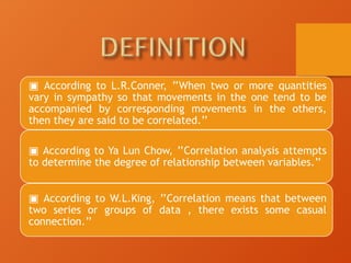
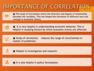
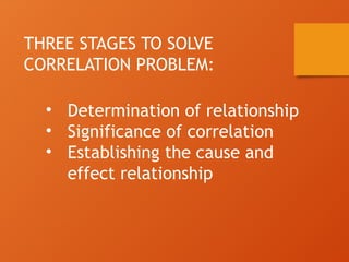
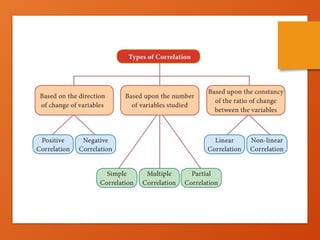
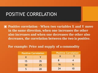
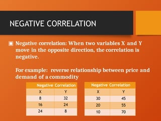
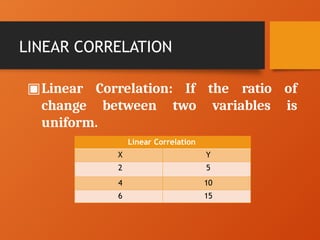
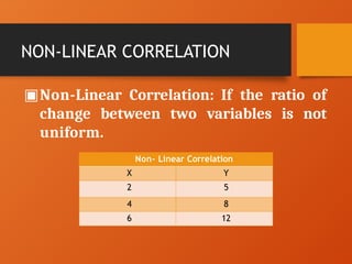
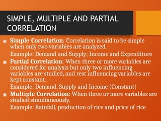
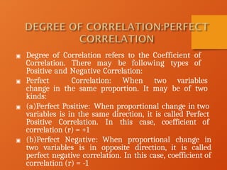
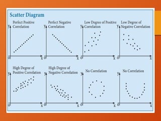
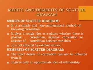
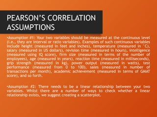
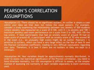
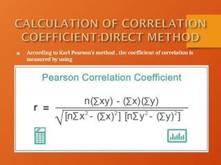
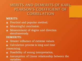
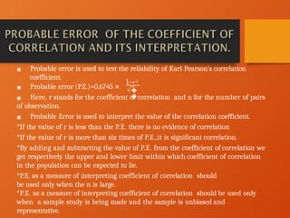
CORRELATION
ANALYSIS
Why do most students who are
good in Mathematics also
perform well in Physics? Why
does blood pressure go with
age? Why do students with high
IQ have good academic
performances? These questions
have something to do with
relationships between
variables.
OBJECTIVES
• Define Correlation Analysis
• Describe relationship
between variables using
degree of correlation
• Solve the value of
correlation coefficient
It is a statistical method or
a statistical technique that
measures the degree of
association between two or more
variables.
▣ According to L.R.Conner, ’’When two or more quantities
vary in sympathy so that movements in the one tend to be
accompanied by corresponding movements in the others,
then they are said to be correlated.’’
▣ According to Ya Lun Chow, ’’Correlation analysis attempts
to determine the degree of relationship between variables.’’
▣ According to W.L.King, ’’Correlation means that between
two series or groups of data , there exists some casual
connection.’’
▣ The study of Correlation shows the direction and degree of relationship
between the variables. This has helped the formation of different laws and
concept in economic theory.
▣ It is very helpful in understanding economic behavior. This is
helpful in studying factors by which economic events are affected.
▣ Study of correlation reduces the range of uncertainties in
matter of prediction.
▣ Helpful in investigation and research.
▣ It is also helpful in policy formulation.
THREE STAGES TO SOLVE
CORRELATION PROBLEM:
• Determination of relationship
• Significance of correlation
• Establishing the cause and
effect relationship
▣ Positive correlation - When two variables X and Y move
in the same direction, when one increases the other
also increases and when one decreases the other also
decreases, the correlation between the two is positive.
For example: Price and supply of a commodity
Positive Correlation
X Y
8 4
16 6
24 10
Positive Correlation
X Y
15 35
10 25
5 20
POSITIVE CORRELATION
▣ Negative correlation: When two variables X and Y
move in the opposite direction, the correlation is
negative.
For example: reverse relationship between price and
demand of a commodity
Negative Correlation
X Y
8 32
16 24
24 8
Negative Correlation
X Y
30 45
20 55
10 70
NEGATIVE CORRELATION
▣Linear Correlation: If the ratio of
change between two variables is
uniform.
Linear Correlation
X Y
2 5
4 10
6 15
LINEAR CORRELATION
▣Non-Linear Correlation: If the ratio of
change between two variables is not
uniform.
Non- Linear Correlation
X Y
2 5
4 8
6 12
NON-LINEAR CORRELATION
SIMPLE, MULTIPLE AND PARTIAL
CORRELATION
▣ Simple Correlation: Correlation is said to be simple
when only two variables are analyzed.
Example: Demand and Supply; Income and Expenditure
▣ Partial Correlation: When three or more variables are
considered for analysis but only two influencing
variables are studied, and rest influencing variables are
kept constant.
Example: Demand, Supply and Income (Constant)
▣ Multiple Correlation: When three or more variables are
studied simultaneously.
Example: Rainfall, production of rice and price of rice
▣ Perfect Correlation
▣ Absence of Correlation or No Correlation
▣ Limited degree of Correlation
(a)High degree of Correlation
(b)Moderate degree of Correlation
(c)Low degree of Correlation
▣ Degree of Correlation refers to the Coefficient of
Correlation. There may be following types of
Positive and Negative Correlation:
▣ Perfect Correlation: When two variables
change in the same proportion. It may be of two
kinds:
▣ (a)Perfect Positive: When proportional change in two
variables is in the same direction, it is called Perfect
Positive Correlation. In this case, coefficient of
correlation (r) = +1
▣ (b)Perfect Negative: When proportional change in
two variables is in opposite direction, it is called
perfect negative correlation. In this case, coefficient of
correlation (r) = -1
▣ Absence of Correlation: If there is no relation
between two variables, it is called no
correlation or absence of correlation. In this
case, coefficient of correlation (r) = 0.
▣ Limited Correlation: Between perfect correlation and no
correlation there is a situation of limited degree of
correlation .In this case the coefficient of correlation (r) is
more than zero and less than one.
▣ There are three types of limited degree of correlation:
▣ (a)High Correlation : When Correlation between two series
is close to one, it is called high degree of correlation. In this
case value of r lies between ±0.75 and ±1.
▣ (b)Moderate Correlation: When Correlation between two series
is neither large nor small, it is called Moderate degree of
Correlation. In this case value of r lies between ±0.25 and ±0.75.
▣ (c)Low Correlation: When the Correlation coefficient between
two series is very small, it is called Low degree Correlation. In
this case value of r lies between 0 and ±0.25.
DEGREE POSITIVE NEGATIVE
Perfect +1 -1
High Between +0.75 and +1 Between -0.75 and -1
Moderate Between +0.25 and +0.75 Between -0.25 and -0.75
Low Between 0 and +0.25 Between 0 and -0.25
Absence of Correlation 0 0
▣ SCATTER DIAGRAM
▣ KARL PEARSON’S COEFFICIENT OF
CORRELATION
▣ COEFFICIENT OF CORRELATION BY RANK
DIFFERENCES
▣ COEFFICIENT OF CONCURRENT
DEVIATION
▣ REGRESSION LINES AND REGRESSION
COEFFICIENT
▣ Scatter Diagram Method: The existence of
Correlation between variables can be shown
graphically by means of a Scatter diagram. It
is obtained by plotting value on a graph paper.
The chart is prepared by measuring X- variable
on horizontal axis and the Y-variable on
vertical axis and all the observations are
plotted on a graph. The cluster points, so
obtained on graph paper is called the Scatter
diagram or dot diagram.
MERITS OF SCATTER DIAGRAM:
▣ It is a simple and non-mathematical method of
knowing correlation.
▣ It gives a rough idea at a glance whether there is
positive correlation, negative correlation or
absence of correlation between variables.
▣ It is not affected by extreme values.
DEMERITS OF SCATTER DIAGRAM:
▣ The exact degree of correlation can not be obtained
from it.
▣ It gives only an approximate idea of relationship.
•The first person to give a mathematical
formula for the measurement of the degree of
relationship between two variables in 1890 was
Karl Pearson.
•Karl Pearson is widely viewed as the founder
of modern statistics. In addition to discovering
numerous statistical concepts, he pushed to
create statistics as a distinct discipline,
founding the first ever university statistics
department and the first academic journal
focused on the field. Unfortunately, like many
intellectuals at the time, his attempts to study
human populations led him to embrace
genocidal politics.
KARL PEARSON
(1857-1936)
•Assumption #1: Your two variables should be measured at the continuous level
(i.e., they are interval or ratio variables). Examples of such continuous variables
include height (measured in feet and inches), temperature (measured in °C),
salary (measured in US dollars), revision time (measured in hours), intelligence
(measured using IQ score), firm size (measured in terms of the number of
employees), age (measured in years), reaction time (measured in milliseconds),
grip strength (measured in kg), power output (measured in watts), test
performance (measured from 0 to 100), sales (measured in number of
transactions per month), academic achievement (measured in terms of GMAT
score), and so forth.
•Assumption #2: There needs to be a linear relationship between your two
variables. Whilst there are a number of ways to check whether a linear
relationship exists, we suggest creating a scatterplot.
PEARSON’S CORRELATION
ASSUMPTIONS
•Assumption #3: There should be no significant outliers. An outlier is simply a case
within your data set that does not follow the usual pattern. For example,
consider a study examining the relationship between test anxiety of 500 students
(where anxiety was measured on a scale of 0-100, with 0 = no anxiety and 100 =
maximum anxiety) and exam performance (on a scale from 0 to 100, with 100 the
top score). If most participants that had an anxiety score of around 70 had an
exam score of around 45, a participant with an anxiety score of 70 who scored 90
in the exam (i.e., an unusually high score) might be an outlier. Pearson's r is
sensitive to outliers, which can have a very large effect on the line of best fit and
the Pearson correlation coefficient, leading to very difficult conclusions regarding
your data. Therefore, it is best if there are no outliers or they are kept to a
minimum.
•Assumption #4: Your variables should be approximately normally distributed. In
order to assess the statistical significance of the Pearson correlation, you need to
have bivariate normality, but this assumption is difficult to assess, so the simpler
method of assessing the normality of each variable separately is more commonly
used.
PEARSON’S CORRELATION
ASSUMPTIONS
▣ A mathematical method for measuring the linear
relationship between the variable X and Y was suggested by
the great biologist and statistician Karl Pearson.
▣ This method is also called Product Moment Method or
Simple Correlation Coefficient.
▣ This method of measuring the coefficient of
correlation is the most popular and is widely used. It
is denoted by “r”, where r is a pure number which
means that r has no unit.
▣ According to Karl Pearson, “Coefficient of
Correlation is calculated by dividing the sum of
products of deviations from their respective means
by their number of pairs and their standard
deviations.”
▣ According to Karl Pearson’s method , the coefficient of correlation is
measured by using
MERITS:
▣ Practical and popular method.
▣ Meaningful conclusion.
▣ Measurement of degree and direction
simultaneously.
DEMERITS:
▣ Greater influence of extreme values.
▣ Calculation process is long and time
consuming.
▣ Possibility of wrong interpretation.
▣ Assumption of Linear relationship between the
variables.
▣ Probable error is used to test the reliability of Karl Pearson’s correlation
coefficient.
▣ Probable error (P.E.)=0.6745 ×
1−𝑟2
�
�
▣ Here, r stands for the coefficient of correlation and n for the number of pairs
of observation.
▣ Probable Error is used to interpret the value of the correlation coefficient.
*If the value of r is less than the P.E. there is no evidence of correlation
*If the value of r is more than six times of P.E.,it is significant correlation.
*By adding and subtracting the value of P.E. from the coefficient of correlation we
get respectively the upper and lower limit within which coefficient of correlation
in the population can be expected to lie.
*P.E. as a measure of interpreting coefficient of correlation should
be used only when the n is large.
*P.E. as a measure of interpreting coefficient of correlation should be used only
when a sample study is being made and the sample is unbiased and
representative.
DciupewdncupiercnuiperhcCORRELATION-ANALYSIS.pptx

DciupewdncupiercnuiperhcCORRELATION-ANALYSIS.pptx

  • 1.
  • 2.
    Why do moststudents who are good in Mathematics also perform well in Physics? Why does blood pressure go with age? Why do students with high IQ have good academic performances? These questions have something to do with relationships between variables.
  • 3.
    OBJECTIVES • Define CorrelationAnalysis • Describe relationship between variables using degree of correlation • Solve the value of correlation coefficient
  • 4.
    It is astatistical method or a statistical technique that measures the degree of association between two or more variables.
  • 5.
    ▣ According toL.R.Conner, ’’When two or more quantities vary in sympathy so that movements in the one tend to be accompanied by corresponding movements in the others, then they are said to be correlated.’’ ▣ According to Ya Lun Chow, ’’Correlation analysis attempts to determine the degree of relationship between variables.’’ ▣ According to W.L.King, ’’Correlation means that between two series or groups of data , there exists some casual connection.’’
  • 6.
    ▣ The studyof Correlation shows the direction and degree of relationship between the variables. This has helped the formation of different laws and concept in economic theory. ▣ It is very helpful in understanding economic behavior. This is helpful in studying factors by which economic events are affected. ▣ Study of correlation reduces the range of uncertainties in matter of prediction. ▣ Helpful in investigation and research. ▣ It is also helpful in policy formulation.
  • 7.
    THREE STAGES TOSOLVE CORRELATION PROBLEM: • Determination of relationship • Significance of correlation • Establishing the cause and effect relationship
  • 9.
    ▣ Positive correlation- When two variables X and Y move in the same direction, when one increases the other also increases and when one decreases the other also decreases, the correlation between the two is positive. For example: Price and supply of a commodity Positive Correlation X Y 8 4 16 6 24 10 Positive Correlation X Y 15 35 10 25 5 20 POSITIVE CORRELATION
  • 10.
    ▣ Negative correlation:When two variables X and Y move in the opposite direction, the correlation is negative. For example: reverse relationship between price and demand of a commodity Negative Correlation X Y 8 32 16 24 24 8 Negative Correlation X Y 30 45 20 55 10 70 NEGATIVE CORRELATION
  • 11.
    ▣Linear Correlation: Ifthe ratio of change between two variables is uniform. Linear Correlation X Y 2 5 4 10 6 15 LINEAR CORRELATION
  • 12.
    ▣Non-Linear Correlation: Ifthe ratio of change between two variables is not uniform. Non- Linear Correlation X Y 2 5 4 8 6 12 NON-LINEAR CORRELATION
  • 13.
    SIMPLE, MULTIPLE ANDPARTIAL CORRELATION ▣ Simple Correlation: Correlation is said to be simple when only two variables are analyzed. Example: Demand and Supply; Income and Expenditure ▣ Partial Correlation: When three or more variables are considered for analysis but only two influencing variables are studied, and rest influencing variables are kept constant. Example: Demand, Supply and Income (Constant) ▣ Multiple Correlation: When three or more variables are studied simultaneously. Example: Rainfall, production of rice and price of rice
  • 14.
    ▣ Perfect Correlation ▣Absence of Correlation or No Correlation ▣ Limited degree of Correlation (a)High degree of Correlation (b)Moderate degree of Correlation (c)Low degree of Correlation
  • 15.
    ▣ Degree ofCorrelation refers to the Coefficient of Correlation. There may be following types of Positive and Negative Correlation: ▣ Perfect Correlation: When two variables change in the same proportion. It may be of two kinds: ▣ (a)Perfect Positive: When proportional change in two variables is in the same direction, it is called Perfect Positive Correlation. In this case, coefficient of correlation (r) = +1 ▣ (b)Perfect Negative: When proportional change in two variables is in opposite direction, it is called perfect negative correlation. In this case, coefficient of correlation (r) = -1
  • 16.
    ▣ Absence ofCorrelation: If there is no relation between two variables, it is called no correlation or absence of correlation. In this case, coefficient of correlation (r) = 0.
  • 17.
    ▣ Limited Correlation:Between perfect correlation and no correlation there is a situation of limited degree of correlation .In this case the coefficient of correlation (r) is more than zero and less than one. ▣ There are three types of limited degree of correlation: ▣ (a)High Correlation : When Correlation between two series is close to one, it is called high degree of correlation. In this case value of r lies between ±0.75 and ±1. ▣ (b)Moderate Correlation: When Correlation between two series is neither large nor small, it is called Moderate degree of Correlation. In this case value of r lies between ±0.25 and ±0.75. ▣ (c)Low Correlation: When the Correlation coefficient between two series is very small, it is called Low degree Correlation. In this case value of r lies between 0 and ±0.25.
  • 18.
    DEGREE POSITIVE NEGATIVE Perfect+1 -1 High Between +0.75 and +1 Between -0.75 and -1 Moderate Between +0.25 and +0.75 Between -0.25 and -0.75 Low Between 0 and +0.25 Between 0 and -0.25 Absence of Correlation 0 0
  • 19.
    ▣ SCATTER DIAGRAM ▣KARL PEARSON’S COEFFICIENT OF CORRELATION ▣ COEFFICIENT OF CORRELATION BY RANK DIFFERENCES ▣ COEFFICIENT OF CONCURRENT DEVIATION ▣ REGRESSION LINES AND REGRESSION COEFFICIENT
  • 20.
    ▣ Scatter DiagramMethod: The existence of Correlation between variables can be shown graphically by means of a Scatter diagram. It is obtained by plotting value on a graph paper. The chart is prepared by measuring X- variable on horizontal axis and the Y-variable on vertical axis and all the observations are plotted on a graph. The cluster points, so obtained on graph paper is called the Scatter diagram or dot diagram.
  • 22.
    MERITS OF SCATTERDIAGRAM: ▣ It is a simple and non-mathematical method of knowing correlation. ▣ It gives a rough idea at a glance whether there is positive correlation, negative correlation or absence of correlation between variables. ▣ It is not affected by extreme values. DEMERITS OF SCATTER DIAGRAM: ▣ The exact degree of correlation can not be obtained from it. ▣ It gives only an approximate idea of relationship.
  • 23.
    •The first personto give a mathematical formula for the measurement of the degree of relationship between two variables in 1890 was Karl Pearson. •Karl Pearson is widely viewed as the founder of modern statistics. In addition to discovering numerous statistical concepts, he pushed to create statistics as a distinct discipline, founding the first ever university statistics department and the first academic journal focused on the field. Unfortunately, like many intellectuals at the time, his attempts to study human populations led him to embrace genocidal politics. KARL PEARSON (1857-1936)
  • 24.
    •Assumption #1: Yourtwo variables should be measured at the continuous level (i.e., they are interval or ratio variables). Examples of such continuous variables include height (measured in feet and inches), temperature (measured in °C), salary (measured in US dollars), revision time (measured in hours), intelligence (measured using IQ score), firm size (measured in terms of the number of employees), age (measured in years), reaction time (measured in milliseconds), grip strength (measured in kg), power output (measured in watts), test performance (measured from 0 to 100), sales (measured in number of transactions per month), academic achievement (measured in terms of GMAT score), and so forth. •Assumption #2: There needs to be a linear relationship between your two variables. Whilst there are a number of ways to check whether a linear relationship exists, we suggest creating a scatterplot. PEARSON’S CORRELATION ASSUMPTIONS
  • 25.
    •Assumption #3: Thereshould be no significant outliers. An outlier is simply a case within your data set that does not follow the usual pattern. For example, consider a study examining the relationship between test anxiety of 500 students (where anxiety was measured on a scale of 0-100, with 0 = no anxiety and 100 = maximum anxiety) and exam performance (on a scale from 0 to 100, with 100 the top score). If most participants that had an anxiety score of around 70 had an exam score of around 45, a participant with an anxiety score of 70 who scored 90 in the exam (i.e., an unusually high score) might be an outlier. Pearson's r is sensitive to outliers, which can have a very large effect on the line of best fit and the Pearson correlation coefficient, leading to very difficult conclusions regarding your data. Therefore, it is best if there are no outliers or they are kept to a minimum. •Assumption #4: Your variables should be approximately normally distributed. In order to assess the statistical significance of the Pearson correlation, you need to have bivariate normality, but this assumption is difficult to assess, so the simpler method of assessing the normality of each variable separately is more commonly used. PEARSON’S CORRELATION ASSUMPTIONS
  • 26.
    ▣ A mathematicalmethod for measuring the linear relationship between the variable X and Y was suggested by the great biologist and statistician Karl Pearson. ▣ This method is also called Product Moment Method or Simple Correlation Coefficient. ▣ This method of measuring the coefficient of correlation is the most popular and is widely used. It is denoted by “r”, where r is a pure number which means that r has no unit. ▣ According to Karl Pearson, “Coefficient of Correlation is calculated by dividing the sum of products of deviations from their respective means by their number of pairs and their standard deviations.”
  • 27.
    ▣ According toKarl Pearson’s method , the coefficient of correlation is measured by using
  • 28.
    MERITS: ▣ Practical andpopular method. ▣ Meaningful conclusion. ▣ Measurement of degree and direction simultaneously. DEMERITS: ▣ Greater influence of extreme values. ▣ Calculation process is long and time consuming. ▣ Possibility of wrong interpretation. ▣ Assumption of Linear relationship between the variables.
  • 29.
    ▣ Probable erroris used to test the reliability of Karl Pearson’s correlation coefficient. ▣ Probable error (P.E.)=0.6745 × 1−𝑟2 � � ▣ Here, r stands for the coefficient of correlation and n for the number of pairs of observation. ▣ Probable Error is used to interpret the value of the correlation coefficient. *If the value of r is less than the P.E. there is no evidence of correlation *If the value of r is more than six times of P.E.,it is significant correlation. *By adding and subtracting the value of P.E. from the coefficient of correlation we get respectively the upper and lower limit within which coefficient of correlation in the population can be expected to lie. *P.E. as a measure of interpreting coefficient of correlation should be used only when the n is large. *P.E. as a measure of interpreting coefficient of correlation should be used only when a sample study is being made and the sample is unbiased and representative.