Downloaded 224 times
![The EOQ Inventory Formula by J. M. Cargal
The Assumptions of the EOQ Model
The underlying assumptions of the EOQ problem can be represented by Figure 1. The idea
is that orders for widgets arrive instantly and all at once. Secondly, the demand for widgets is
perfectly steady. Note that it is relatively easy to modify these assumptions; Hadley and Whitin
[1963] cover many such cases. Despite the fact that many more elaborate models have been
constructed for inventory problem the EOQ model is by far the most used.
Figure 1 The EOQ Process
An Incorrect Solution
Solving for the EOQ, that is the quantity that minimizes total costs, requires that we
formulate what the costs are. The order period is the block of time between two consecutive orders.
The length of the order period, which we will denote by P, is Q/D. For example, if the order
quantity is 20 widgets and the rate of demand is five widgets per day, then the order period is 20/5,
or four days. Let Tp be the total costs per order period. By definition, the order cost per order period
will be C. During the order period the inventory will go steadily from Q, the order amount, to zero.
Hence the average inventory is Q/2 and the inventory costs per period is the average cost, Q/2, times
the length of the period, Q/D. Hence the total cost per period is:
Q Q Q2 h
TP C h C
2 D 2D
If we take the derivative of Tp with respect to Q and set it to zero, we get Q = 0. The problem is
solved by the device of not ordering anything. This indeed minimizes the inventory costs but at the
small inconvenience of not meeting demand and therefore going out of business. This is what many
people, perhaps most people do, when trying to solve for the EOQ the first time.
The Classic EOQ Derivation
The first step to solving the EOQ problem is to correctly state the inventory costs formula.
This can be done by taking the cost per period Tp and dividing by the length of the period, Q/D, to
get the total cost per unit time, Tu:
CD Qh
Tu
Q 2
2](https://image.slidesharecdn.com/theeoqformula-120410040821-phpapp01/75/The-EOQ-Formula-2-2048.jpg)
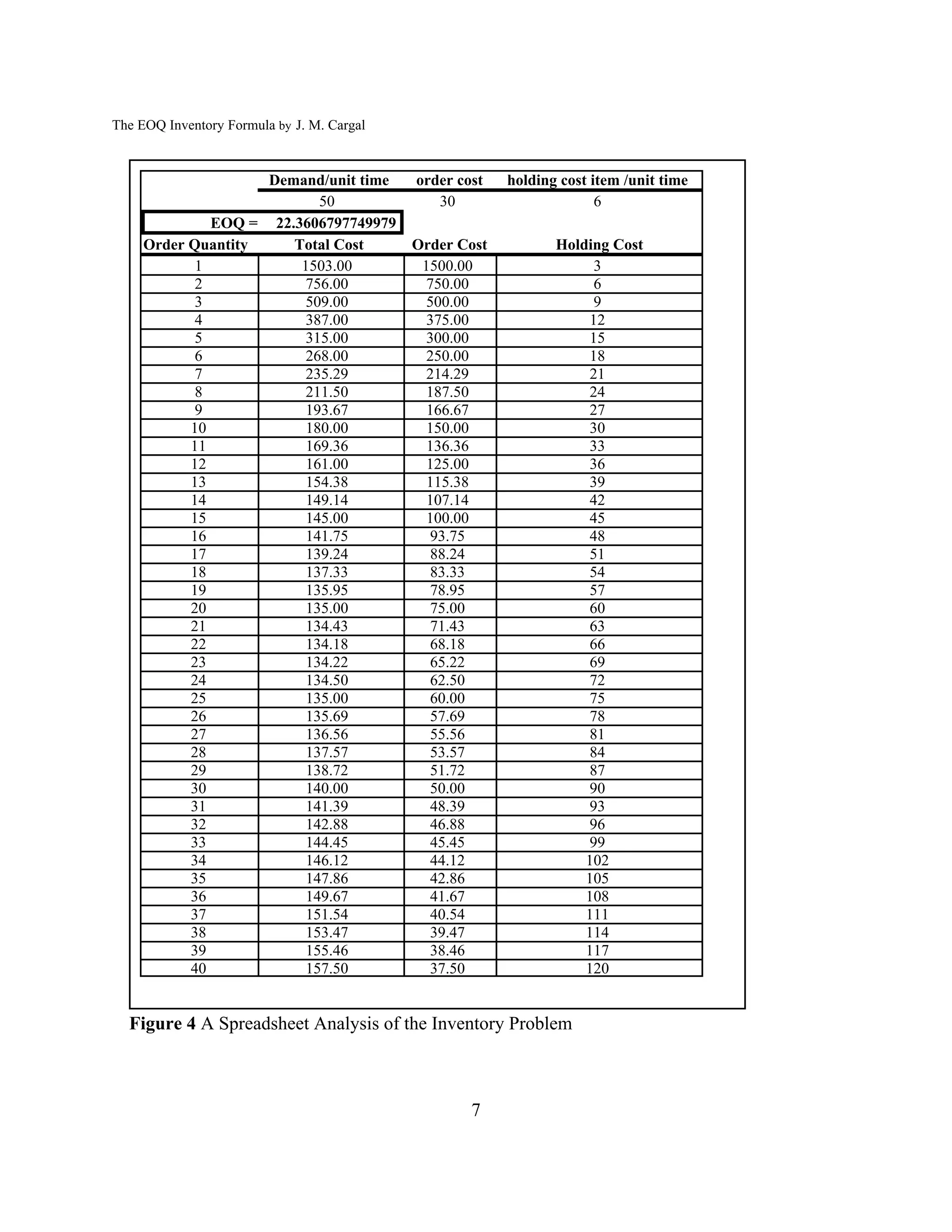

The document discusses the EOQ (economic order quantity) inventory formula. It begins by explaining the variables and assumptions of the EOQ model, which determines the optimal order quantity to minimize total inventory costs. It then discusses how the formula can be derived by setting the derivatives of total cost equations to zero. Finally, it explains that while the EOQ assumptions are unrealistic, the formula still works well due to cost functions being relatively flat near the optimum, and spreadsheets now allow evaluating costs without using the formula.


![[231005] - 02. Basic EOQ & EPQ.docx](https://cdn.slidesharecdn.com/ss_thumbnails/231005-02-231022023204-c5a04445-thumbnail.jpg?width=640&height=640&fit=bounds)


