Download to read offline
![IEOR4000: Production Management Professor Guillermo Gallego
Lecture 2 September 9, 2004
Lecture Plan
1. The EOQ and Extensions
2. Multi-Item EOQ Model
1 The EOQ and Extensions
This section is devoted to the Economic Production Quantity (EPQ) model, its specialization to the
Economic Order Quantity (EOQ) model and its extension to allow backorders. The next section
deals with multiple products. The primary driver to hold inventories is the presence of a fixed pro-
duction/ordering cost that is incurred every time a positive number of units are produced/ordered.
We wish to determine the number of units to produce/order every time the fixed production/ordering
cost is incurred. Producing/ordering in large quantities reduce the average fixed production/ordering
cost. What prevents the production/ordering quantities from becoming too large is that it costs
money to hold inventories. Inventory costs include the cost of storage and insurance and the cost of
capital tied up in inventory. The EPQ balances the average fixed ordering cost (that decreases with
large orders) and the average inventory holding cost (that increases with large orders).
We will assume that demand is constant and continuous over an infinite horizon. We will also
assume a constant, continuous, production rate. The objective is to minimize the average cost.
Data:
K set up or ordering cost,
c unit production cost,
h holding cost,
λ demand rate,
µ production rate.
The holding cost is often model as h = Ic where I represents the inventory carrying cost per
unit per unit time and includes the cost of capital per unit per unit time. Let ρ = λ/µ. We assume
ρ ≤ 1, since otherwise the production capacity is not enough to keep up with demand.
Since we have assumed that production and demand rates are constant and costs are stationary,
it makes intuitive sense to produce/order in cycles of equal lengths and to start/end each cycle with
zero inventory. This last property is know as the Zero Inventory Property (ZIP) and can be formally
verified. Let T denote the cycle length. The cycle length is the time between consecutive orders; it
is also called the order/reorder interval. We want to express the average cost a(T ) as a function of
T and then select T to minimize a(T ). We could have also chosen the production/order quantity
Q = λT as the decision variable. The advantage of using a time variable is apparent when dealing
with multiple items, where time provides a unified variable.
Let I(t) denote the inventory at time t. We will assume that I(0) = 0, and by design we want
I(T ) = 0. At time zero we start production at rate µ. We need to determine when to stop production
so that I(T ) = 0. Since λT units are demanded over the interval [0, T ], it takes λT = ρT units of
µ
time to produce λT units at rate µ. Because demand is constant at rate λ, inventory accumulates
at rate µ − λ over the interval [0, ρT ] reaching a peak equal to (µ − λ)ρT = λ(1 − ρ)T at time ρT .
Since production stops at time ρT , inventory decreases at rate λ over the interval [ρT, T ] reaching
zero at time T .
Let us now compute the average inventory over the interval [0, T ]. Formally, this is equal to
T
1
I(t)dt.
T 0
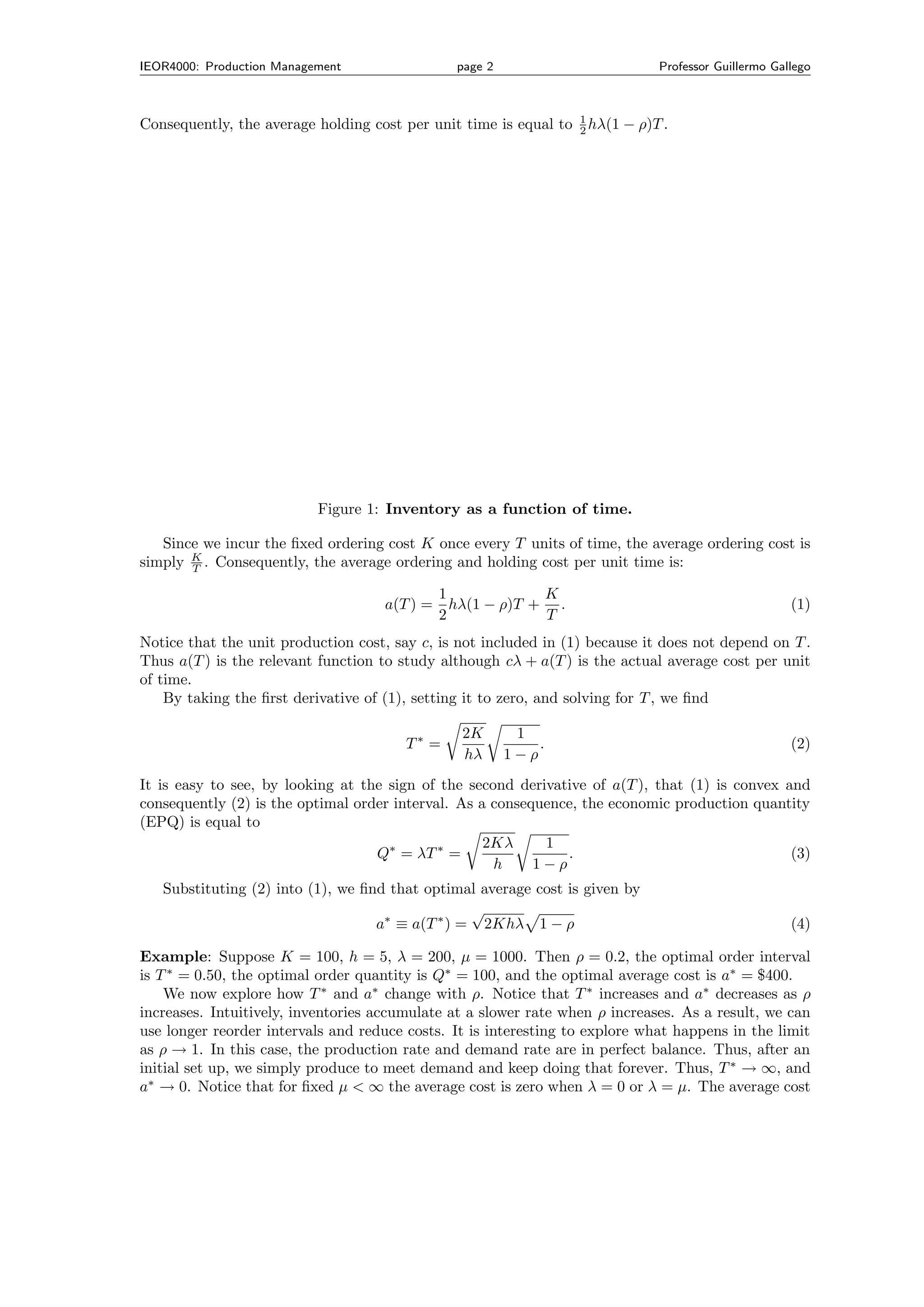
The function I(t) forms a triangle that repeats ever T units of time. The base of each triangle is T
and the height is λ(1 − ρ)T . It follows that
T
1 11 1
I(t)dt = λ(1 − ρ)T 2 = λ(1 − ρ)T.
T 0 T2 2](https://image.slidesharecdn.com/lect02-121202055129-phpapp02/75/Lect-02-1-2048.jpg)
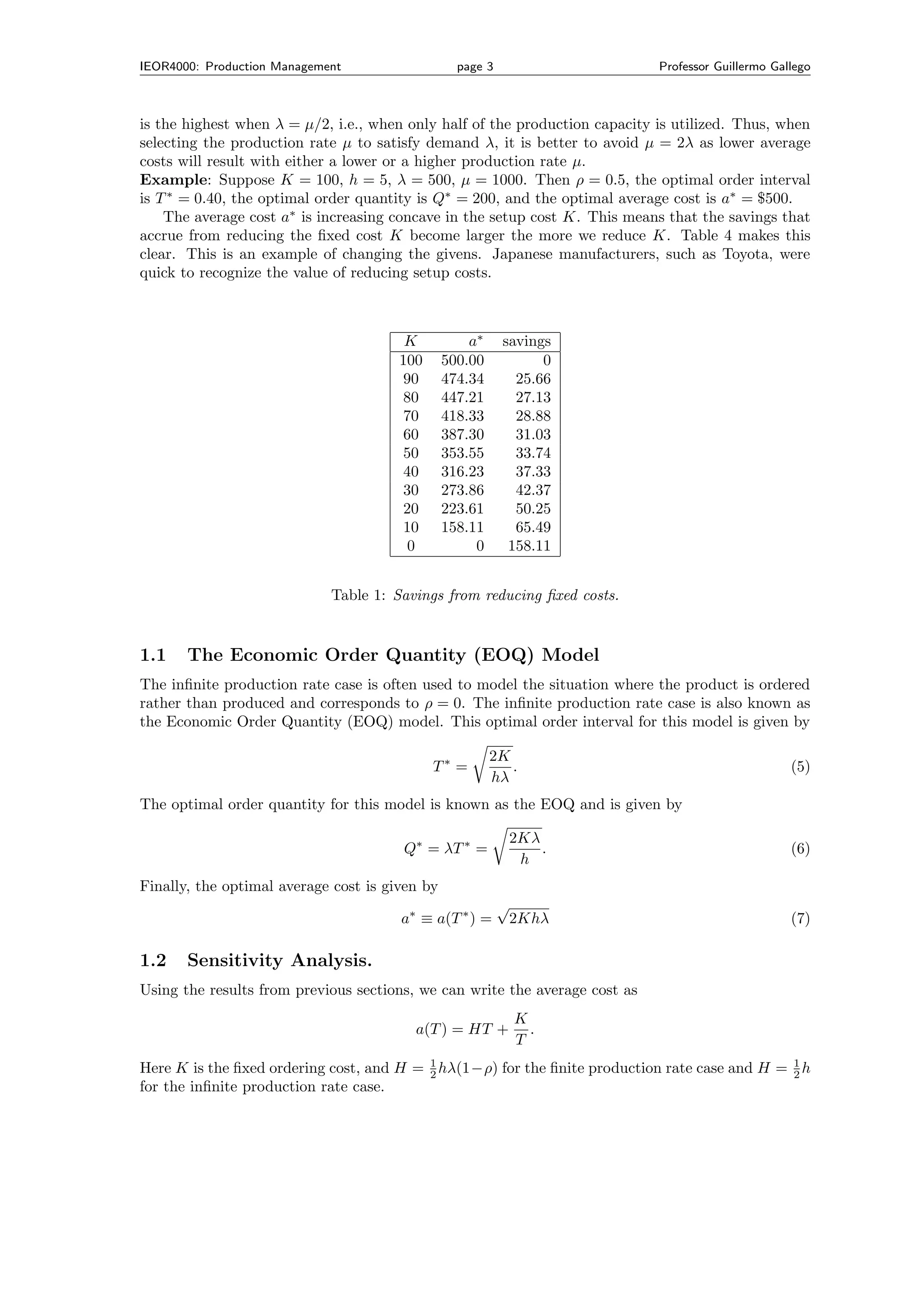

The document summarizes the economic production quantity (EPQ) model and its extensions. It discusses: 1) The EPQ model balances fixed ordering costs and inventory holding costs to determine optimal production/order quantities and intervals. 2) The economic order quantity (EOQ) model is a special case where production rate is infinite and demand is met through ordering. 3) Sensitivity analysis shows how the optimal solutions change with different parameters like production rate and setup costs.