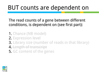
Downloaded 259 times


![Normalize for library size
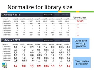
Original library size * scale factor = effective library size
DESeq will multiply original counts by the sample
scaling factor.
DESeq: This normalization method [14] is included in the DESeq Bioconductor package (version 1.6.0) [14] and is based on the hypothesis that most genes are not DE. A DESeq scaling
factor for a given lane is computed as the median of the ratio, for each gene, of its read count
over its geometric mean across all lanes. The underlying idea is that non-DE genes should have
similar read counts across samples, leading to a ratio of 1. Assuming most genes are not DE, the
median of this ratio for the lane provides an estimate of the correction factor that should be
applied to all read counts of this lane to fulfill the hypothesis
DESeq computes a scaling factor for a given sample by computing the median of the ratio, for each gene, of its
read count over its geometric mean across all samples. It then uses the assumption that most genes are not DE
and uses this median of ratios to obtain the scaling factor associated with this sample.
http://www.ncbi.nlm.nih.gov/pmc/articles/PMC3426807/](https://image.slidesharecdn.com/5-140123140706-phpapp02/85/RNA-seq-for-DE-analysis-detecting-differential-expression-part-5-13-320.jpg)


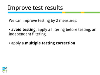


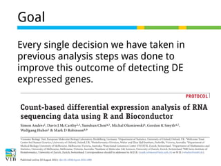
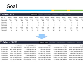
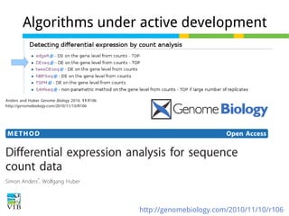
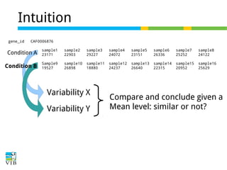
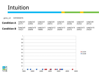
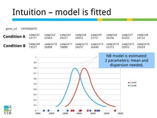
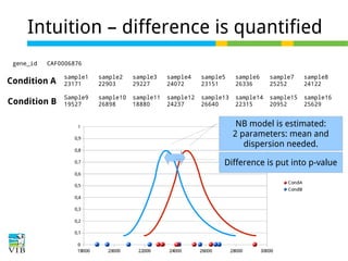
This document outlines the methodology for detecting differentially expressed genes using RNA-seq data analysis, emphasizing the use of count tables to assign p-values indicating the likelihood of differences between conditions. It discusses normalization techniques, specifically through the DESeq package, to adjust for library size and employs statistical models to accurately estimate dispersion and improve testing outcomes. The presentation also highlights the importance of filtering out low-count genes and applying multiple testing corrections to control the false discovery rate.