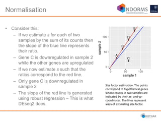
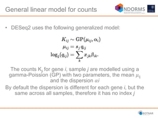
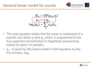
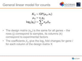
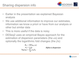
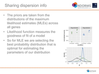
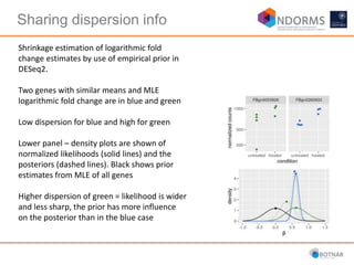
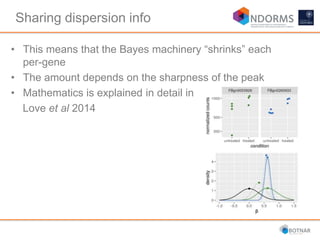
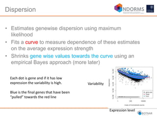
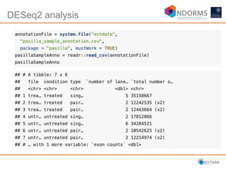
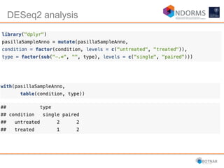
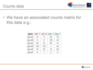
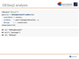
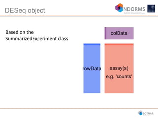
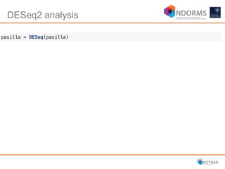
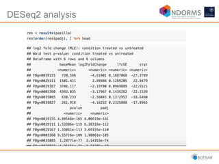
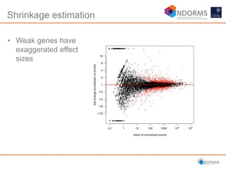
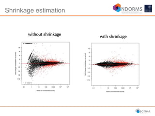
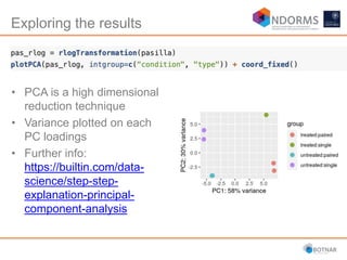
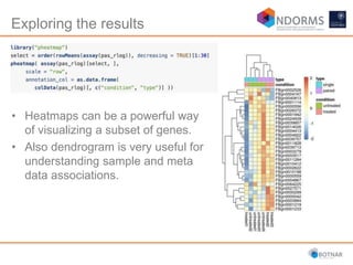
DESeq2 is used to analyze differential expression from RNA-seq count data using a generalized linear model. It models counts using a gamma-Poisson distribution and estimates dispersion using empirical Bayes shrinkage. Key steps include normalizing counts, estimating dispersion, fitting the linear model, and using Wald and likelihood ratio tests to identify differentially expressed genes while controlling the false discovery rate. Results can be explored using plots of p-values, mean-variance trends, ordination plots, and heatmaps to visualize sample relationships and differentially expressed genes.

1. Understanding how to analyse bulk
transcriptomic data using DESEq2
Taken largely from
Modern statistics for modern biology
https://www.huber.embl.de/msmb/

2. Frequentist statistics
• A type of statistical inference that draws conclusions
from sample data by emphasizing the frequency or
proportion of the data.

3. Generative model
• All the parameters of the model are known
• Given an observable variable X and a target variable Y, a
generative model is a statistical model of the join
probability distribution on, P(X,Y), P(X|Y = y).
probability of Y given X
X has already occurred and has been measured

4. Probability distributions
• Probability distribution is a mathematical function that
gives the probabilities of occurrence of different possible
outcomes.
• Mathematical description of the probabilities of events
• Determined empirically from a distribution of data.
• There are some commonly observed distributions –
grouped by the process that they are related to

5. Normal (Gaussian) distribution
• Most important distribution – central limit theorem.
𝜇 mean
𝜎 standard deviation
Probability density function:

6. Log normal distribution
• Probability distribution of a
random variable whose
logarithm is normally
distributed.
• Y = ln(X) has a normal
distribution

7. • a discrete probability distribution that expresses the
probability of a given number of events occurring in a
fixed interval of time or space if these events occur with
a known constant mean rate and independently of the
time since the last event
Possion distribution

8. Bernoulli distribution
• Discrete probability distribution of a
random variable

9. Negative binomial distribution
• RNA-seq counts distribution

10. Statistical modelling
• Once you have a generative model and you have the
parameters to define the probabilities we can start
decision making.
• Goodness of fit – to identify dist
• Statistical detective
We start with data X and use
this to estimate the
parameters of a distribution.
These estimates are donated
by Greek letters and a hat.

11. Rootograms
• Red is theoretical distribution
• Bottom of bar should align with horizontal
• Assess goodness of fit

12. Bayesian statistics
• A method of statistical inference in which Bayes theorem
is used to update the probability for a hypothesis as
more evidence or information becomes available.
• Practical approach where a prior and posterior
distribution are used to model.
• Prior – probability that would express ones belief before
evidence is taken into account. This unknown would
maybe be a parameter of the model or a latent variable
rather than an observable variable.
• Posterior – random variable conditional on the evidence
obtained for an experiment after the relevant evidence is
taken into account

13. Bayesian statistics
• We use probability distributions to express our
knowledge about the parameters, and then use data to
update our knowledge.
• For example, shifting the distributions and making them
more narrow (more to come later).

14. High-throughput count data
• Challenges:
– Large dynamic range - 0 to millions. (heteroscedasticity).
– Non negative integers with uneven distributions – normal or log-
normal distributions may not fit.
– We need to understand the sampling biases and correct.
– Small sample size makes estimation of dispersion difficult.

15. Normalisation
• Normalisation can be misleading term
• Nothing to do with normal distribution
• The aim is to identify sources of bias and take them into
account
• For RNA-seq that’s usually library size (number of reads
for each sample)

16. Normalisation

17. Normalisation
• Consider this:
– If we estimate s for each of two
samples by the sum of its counts then
the slope of the blue line represents
their ratio.
– Gene C is downregulated in sample 2
while the other genes are upregulated
– If we now estimate s such that the
ratios correspond to the red line.
– Only gene C is downregulated in
sample 2
– The slope of the red line is generated
using robust regression – This is what
DEseq2 does.
Size factor estimation. The points
correspond to hypothetical genes
whose counts in two samples are
indicated by their xx- and yy-
coordinates. The lines represent
ways of estimating size factor.

18. Dispersion
• Fragments are molecules being sequenced (equates to
cDNA molecules).
• A sequencing library of n1 fragments corresponding to
gene 1, n2 corresponding to gene 2.
• A total library size is n = n1 + n2 + ..
• We submit the sample for sequencing and determine the
identity of r randomly sampled fragments.

19. Dispersion
• The number of genes is in the tens of thousands
• The value of n (fragments) depends on the amount of
cells that were used to prepare the lib, which could
potentially be billions
• The number of reads r is usually in the tens of millions

20. Dispersion
• A read is the sequence obtained from a fragment.
• Probability that a given read maps to the ith gene is:
– pi = ni/n
• We can model the number of reads for gene i by a
Poission distribution
• The rate of the Poission process is the product of pi, the
initial proportion of fragments for the ith gene, times r
(number of reads):
– 𝜆𝑖 = rp𝑖
– 𝜆𝑖 is the passion parameter (lambda usually
represents this)

21. Dispersion
• In practice we aren’t usually interested in modelling the
counts of the single library but between libraries
• That’s the difference between control and treatment
• It turns out that replicates vary more than the Poission
distribution
• We need to model this so we instead use a Gamma-
Poission (aka. Negative binomial) distribution which
better suits our modelling needs

22. Dispersion

23. We are now ready to fit a model (GLM)
But before GLM we need to understand
linear modelling

24. Linear models
• We perform an siRNA knockdown of CTLA-4 gene. We
also want to study the effect of a drug X.
• We treat cells with neg control, siRNA alone, drug X
alone or both:
y is the experimental measurement of interest i.e. the transformed expression
level of a gene
The coefficient 𝛽0 is the base level of the measurement in control (a.k.a. the
intercept)
𝓍1 and 𝓍2 are binary variables.
𝓍1 Takes value 1 if siRNA is administered
𝓍2 indicated whether drug was administered

25. Linear models
• If only siRNA is used: x1 = 1 and x2 = 0. equation
simplifies to:
• 𝛽1 represents difference between treatment and control.
If measurements are on log scale then:
• This is the logarithmic change due to treatment with
siRNA

26. Linear models
• What if we treat with both drug and siRNA
• x1 = 1 and x2 = 1
• This means that 𝛽12 is the difference between the
observed outcome, y, and the outcome from the
individual treatments, obtained by adding to the baseline
the effect of siRNA alone (𝛽1) and of drug alone (𝛽2).
• 𝛽12 is called the interaction effect of siRNA and drug.

27. Design matrix
• We can encode an experimental design in a matrix:
• The columns represent experimental factors and rows
represent the different experimental conditions

28. Noise and replicates
• To estimate noise you need replicates
• Assessment of uncertainty of our estimated 𝛽s
• Extend equation:
Added the index j and a new term 𝜀j
The index now counts over our individual replicate experiments e.g. if for each of
the four conditions we perform three replicates, then j counts from 1 to 12.
The design matrix has 12 rows, and xjk is the value of the matrix in its jth row and
kth column

29. Noise and replicates
• But what is 𝜀j?
• This is something we call the residuals and absorbs the
differences between replicates
• But we need to take into account the system of twelve
equations (top equation), we have more variables (12
epsilons and four betas)
• We can address this by minimizing the sum of the squared
residuals:

30. General linear model for counts
• The above equation models the the expected value of
the outcome y, as a linear function of the design matrix,
and its fitted to the data according to the least sum of
squares
• We now want to generalize these assumptions

31. • Modelling data on a transformed scale:
– It can be more fruitful to consider data on a scaled level than its
natural scale level – this can be generalized
• Error distributions:
– Other generalized concerns are the minimization criteria
– Generalization can make is to use a different probabilistic model
than the normal distribution – in our case we know that we can
deal with our counts data using a gamma-Poission distribution
(negative binomial distribution)
General linear model for counts

32. • DESeq2 uses the following generalized model:
The counts Kji for gene i, sample j are modelled using a
gamma-Poission (GP) with two parameters, the mean 𝜇ij
and the dispersion 𝛼i
By default the dispersion is different for each gene i, but the
same across all samples, therefore it has no index j
General linear model for counts

33. • The next equation states that the mean is composed of a
specific size factor sj and qij, which is proportional to the
true expected concentration in fragments (sequencing
reads) for gene i in sample j
• qij – is given by the linear model in third equation by the
link function, log2
General linear model for counts

34. • The design matrix (xjk) is the same for all genes – the
rows (j) correspond to samples, its columns (k)
correspond to experimental factors
• The coefficients 𝛽ik give the log2 fold changes for gene i
for each column of the design matrix X
General linear model for counts

35. Sharing dispersion
• In RNA-seq you typically only have a few replicates
– Difficult to estimate within group variability
• Solution is to pool information across genes which are
expressed at a similar level
– Assumes strength of similar average expression strength have
similar dispersion

36. Sharing dispersion info
• Earlier in the presentation we explained Bayesian
analysis
• We use additional information to improve our estimates,
information we know a priori or have from our analysis or
other but similar data
• This is more useful if the data is noisy
• DESeq2 uses an empirical Bayes approach for the
estimation of dispersion parameters (the 𝛼s) and
optionally the logarithmic fold changes (the 𝛽s)
Alpha is dispersion

37. • The priors are taken from the
distributions of the maximum
likelihood estimates (MLEs) across
all genes
• Likelihood function measures the
goodness of fit of a model
• So for MLE we are selecting the
best probability distribution that is
optimal for estimating the
parameters of our distribution
Sharing dispersion info

38. Sharing dispersion info
Shrinkage estimation of logarithmic fold
change estimates by use of empirical prior in
DESeq2.
Two genes with similar means and MLE
logarithmic fold change are in blue and green
Low dispersion for blue and high for green
Lower panel – density plots are shown of
normalized likelihoods (solid lines) and the
posteriors (dashed lines). Black shows prior
estimates from MLE of all genes
Higher dispersion of green = likelihood is wider
and less sharp, the prior has more influence
on the posterior than in the blue case

39. Sharing dispersion info
• This means that the Bayes machinery “shrinks” each
per-gene
• The amount depends on the sharpness of the peak
• Mathematics is explained in detail in
Love et al 2014

40. Dispersion
• Estimates genewise dispersion using maximum
likelihood
• Fits a curve to measure dependence of these estimates
on the average expression strength
• Shrinks gene wise values towards the curve using an
empirical Bayes approach (more later)
Expression level
Variability
Each dot is gene and if it has low
expression the variability is high.
Blue is the final genes that have been
“pulled” towards the red line

41. • Once a GLM is fitted then a wald test is
performed for the treatment coefficient
Wald test

42. • Analyze all levels of a factor at once
• LRT which is used to identify any genes that show
change in expression across the different levels
• This type of test can be especially useful in analyzing
time course experiments
LRT test

43. DESeq2 analysis

44. DESeq2 analysis

45. Counts data
• We have an associated counts matrix for
this data e.g.:

46. DESeq2 analysis

47. DESeq object
Based on the
SummarizedExperiment class

48. DESeq2 analysis

49. DESeq2 analysis

50. Exploring the results
• There are four main plots that explain a lot about
your data:
– The histogram of p values
– The MA plot
– An ordination plot
– A heatmap

51. Exploring the results
• The left hand peak is differentially
expressed genes.
• Background is right hand.
• Pvalue < 0.01 ~ 990 genes.
• The background is around 100
genes.
• This suggests 10% FDR.
• A shifted background distribution
could indicate batch effects.

52. • Fold changes vs mean of
size-factor normalized
counts
• Log scale for both axes
• Blue points are significant
genes
Exploring the results

53. Shrinkage estimation
• Weak genes have
exaggerated effect
sizes

54. Shrinkage estimation

55. • Fit GLM for all genes without shrinkage
• Estimate normal empirical-Bayes prior
from non-intercept coefficients
• Add log prior to the GLMs log likelihoods
results in a ridge penalty
• Fit GLMs again now with penalized
likelihoods to get shrunken coefficients
Shrinkage estimation

56. • PCA is a high dimensional
reduction technique
• Variance plotted on each
PC loadings
• Further info:
https://builtin.com/data-
science/step-step-
explanation-principal-
component-analysis
Exploring the results

57. • Heatmaps can be a powerful way
of visualizing a subset of genes.
• Also dendrogram is very useful for
understanding sample and meta
data associations.
Exploring the results

58. Dealing with outliers
• Sometimes data can contain very large counts that
appear unrelated to the experimental design
• Outliers arise for many reasons – technical experimental
artefacts
• A diagnostic test for outliers is Cook’s distance
• Cook’s distance is a measure of how much a single
sample is influencing the fitted coefficients for a gene