Downloaded 49 times


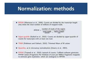
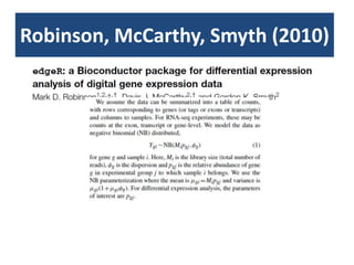
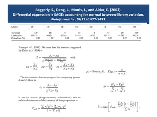
![Normalization (2)Within-library normalization allows quantification of expression levels of each gene relative to other genes in the sample. Because longer transcripts have higher read counts (at the same expression level), a common method for within-library normalization is to divide the summarized counts by the length of the gene [32,34]. The widely used RPKM (reads per kilobase of exon model per million mapped reads) accounts for both library size and gene length effects in within-sample comparisons. When testing individual genes for DE between samples, technical biases, such as gene length and nucleotide composition, will mainly cancel out because the underlying sequence used for summarization is the same between samples. However, between-sample normalization is still essential for comparing counts from different libraries relative to each other. The simplest and most commonly used normalization adjusts by the total number of reads in the library [34,51], accounting for the fact that more reads will be assigned to each gene if a sample is sequenced to a greater depth.](https://image.slidesharecdn.com/110512presentacionantoniminarro-110512084740-phpapp02/85/EiB-Seminar-from-Antoni-Minarro-Ph-D-14-320.jpg)

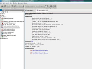


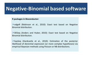
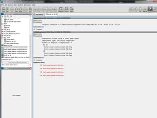
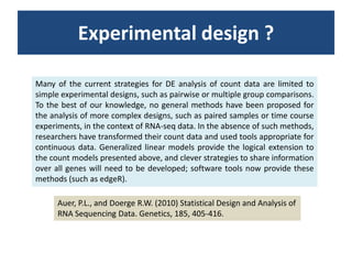
![baySeq (Hardcastle et al., 2010): Estimation of the posterior likelihood of dierential expression (or more complex hypotheses) via empirical Bayesian methods using Poisson or NB distributions.CLC GenomicsWorkbenchapproach19.4.2.1 Kal et al.'s test (Z-test) Kal et al.'s test [Kal et al., 1999] compares a single sample against another single sample, and thus requires that each group in you experiment has only one sample. The test relies on an approximation of the binomial distribution by the normal distribution [Kal et al., 1999]. Considering proportions rather than raw counts the test is also suitable in situations where the sum of counts is different between the samples. 19.4.2.2 Baggerley et al.'s test (Beta-binomial) Baggerley et al.'s test [Baggerly et al., 2003] compares the proportions of counts in a group of samples against those of another group of samples, and is suited to cases where replicates are available in the groups. The samples are given different weights depending on their sizes (total counts). The weights are obtained by assuming a Beta distribution on the proportions in a group, and estimating these, along with the proportion of a binomial distribution, by the method of moments. The result is a weighted t-type test statistic.](https://image.slidesharecdn.com/110512presentacionantoniminarro-110512084740-phpapp02/85/EiB-Seminar-from-Antoni-Minarro-Ph-D-36-320.jpg)
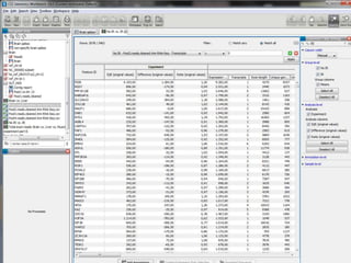
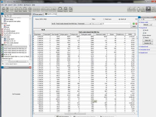
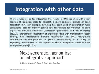
![Resolució amb edgeR> library(edgeR)> set.seed(101)> n <- 200> lib.sizes <- c(40000, 50000, 38000, 40000)> p <- runif(n, min = 1e-04, 0.001)> mu <- outer(p, lib.sizes)> mu[1:5, 3:4] <- mu[1:5, 3:4] * 8> y <- matrix(rnbinom(4 * n, size = 4, mu = mu), nrow = n)> rownames(y) <- paste("tag", 1:nrow(y), sep = ".")> y[1:10, ] [,1] [,2] [,3] [,4]tag.1 15 13 117 77tag.2 3 4 49 33tag.3 25 56 302 332tag.4 40 13 271 91tag.5 13 3 51 56tag.6 14 7 31 18tag.7 16 39 19 9tag.8 6 28 6 6tag.9 10 42 80 14tag.10 33 25 5 27> d <- DGEList(counts = y, group = rep(1:2, each = 2), lib.size = lib.sizes)> d <- estimateCommonDisp(d)> de.common <- exactTest(d)Comparison of groups: 2 - 1 > topTags(de.common)Comparison of groups: 2 - 1 logConclogFCPValue FDRtag.184 -13.636760 -5.236853 6.112570e-05 0.005195714tag.2 -11.769438 3.766465 6.405229e-05 0.005195714tag.3 -8.550981 3.214682 7.793571e-05 0.005195714tag.4 -9.188394 2.911743 3.300004e-04 0.013214944tag.1 -10.135230 2.984351 3.303736e-04 0.013214944tag.5 -10.944756 2.868619 1.035516e-03 0.034517212tag.105 -10.693557 2.618355 2.337750e-03 0.066792856tag.164 -11.253348 -2.209660 1.090272e-02 0.233310771tag.14 -11.258031 2.238669 1.090272e-02 0.233310771tag.123 -13.277812 -2.756096 1.166554e-02 0.233310771> >](https://image.slidesharecdn.com/110512presentacionantoniminarro-110512084740-phpapp02/85/EiB-Seminar-from-Antoni-Minarro-Ph-D-41-320.jpg)

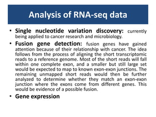
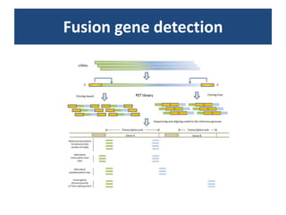
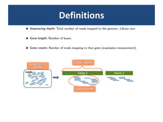
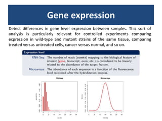
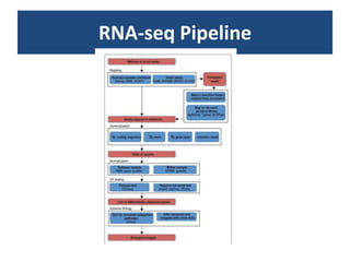
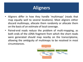
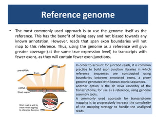
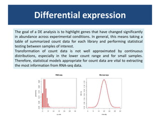
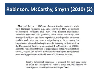
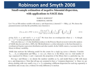
RNA-seq, or whole transcriptome shotgun sequencing, involves high-throughput sequencing of cDNA to analyze RNA content, particularly for cancer research and microbiology. The process includes single nucleotide variation discovery, fusion gene detection, and differential expression analysis, with statistical models essential for accurate interpretation of count data. Various methods, including normalization techniques and different statistical distributions (such as Poisson and negative binomial), are used to account for biological variability in RNA-seq datasets.


![[DigiHealth 22] Budget friendly sample sizes for genomics research - Ognjen M...](https://cdn.slidesharecdn.com/ss_thumbnails/ognjen-budgetfriendlysamplesizesforgenomicsresearch-novideo-221129214128-09e5f81f-thumbnail.jpg?width=640&height=640&fit=bounds)


