Downloaded 34 times
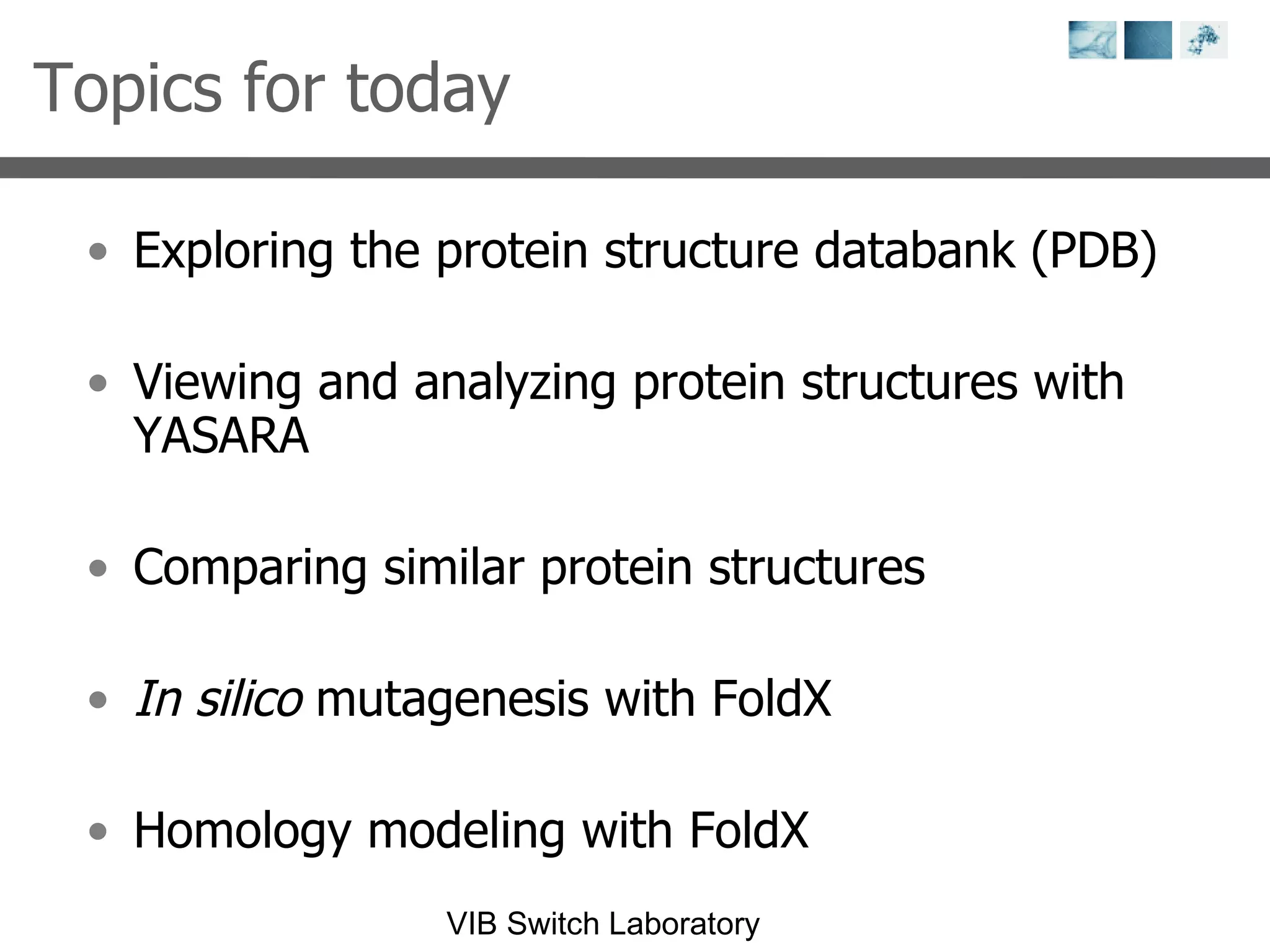
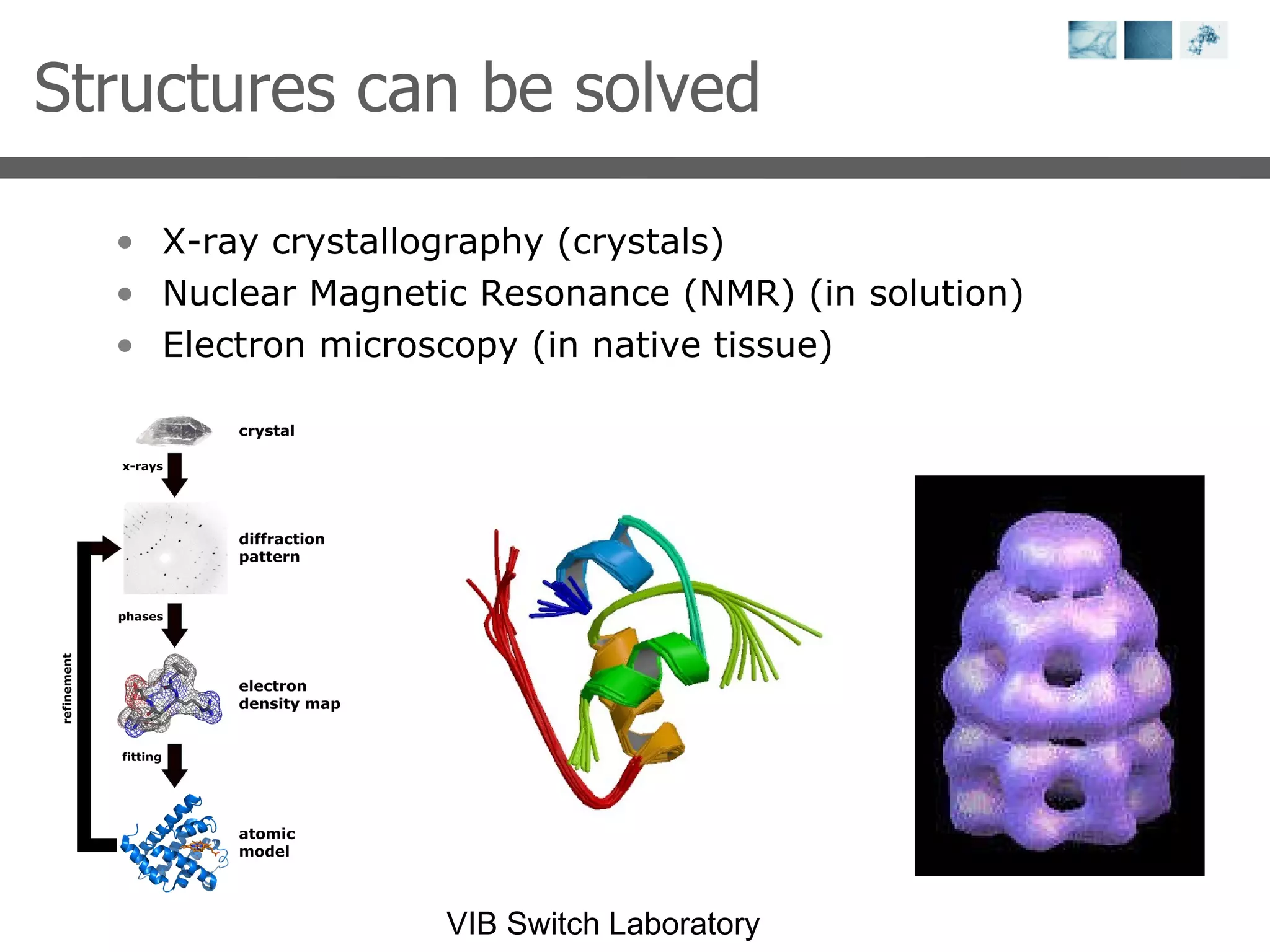
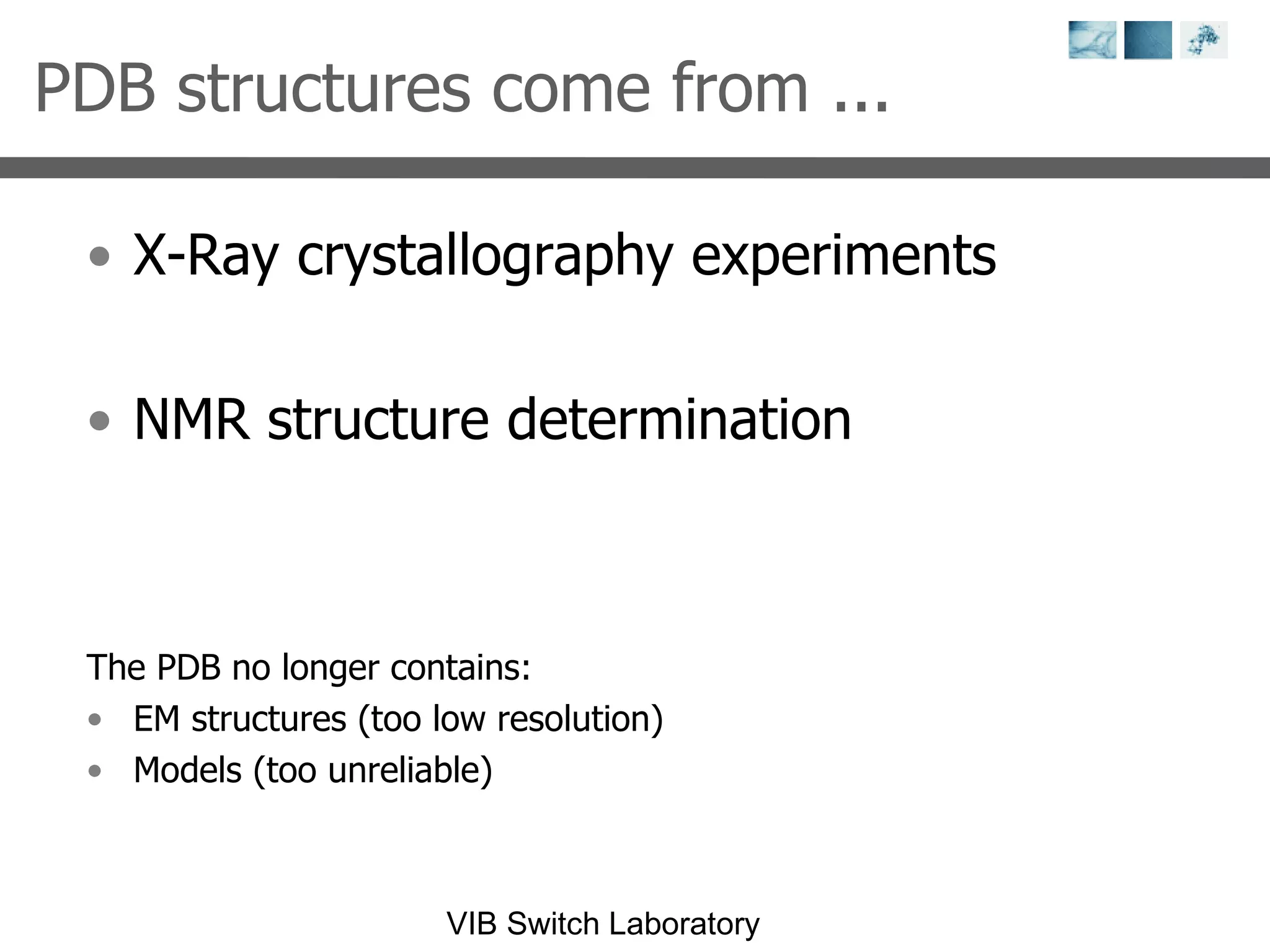
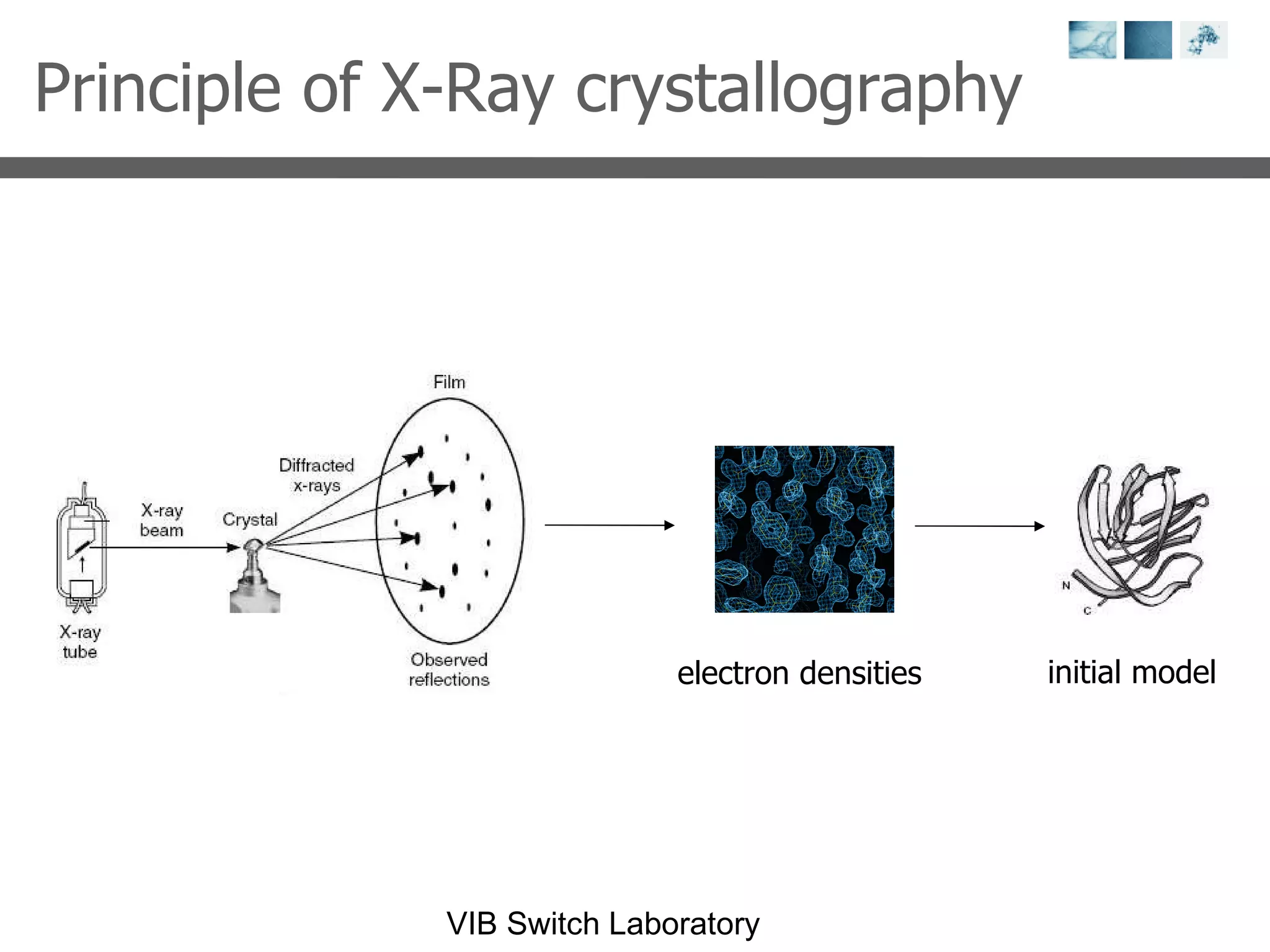
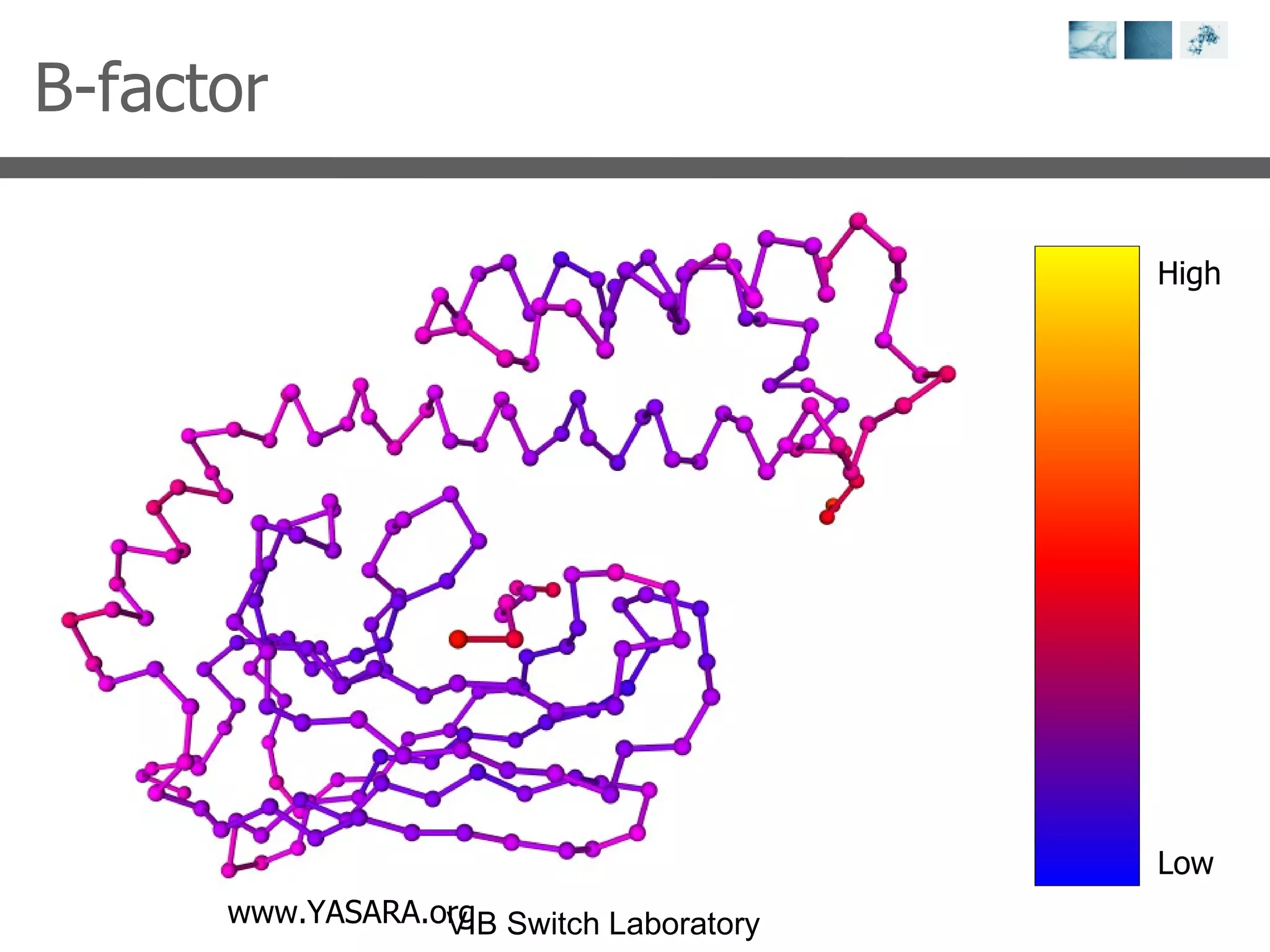
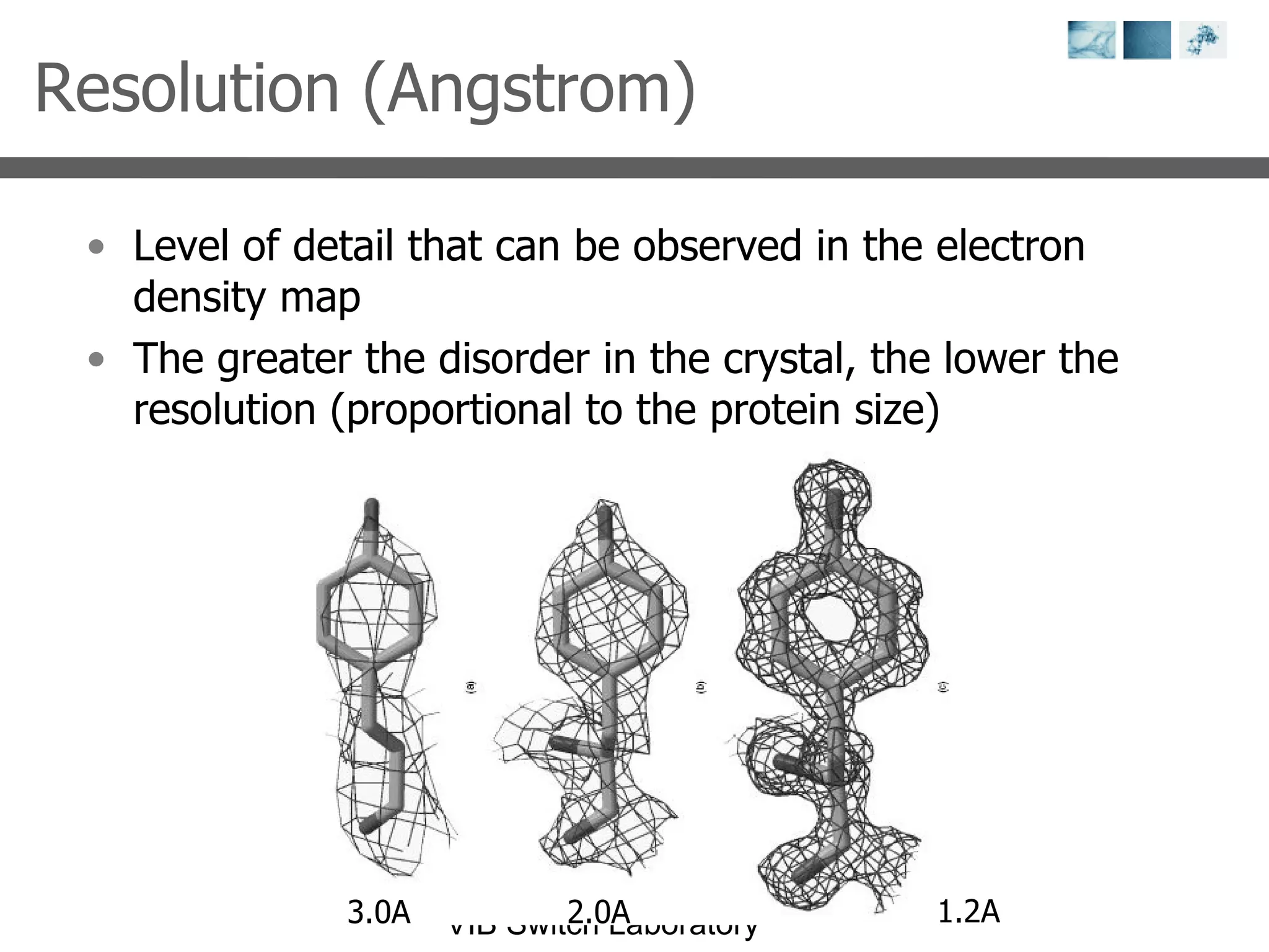
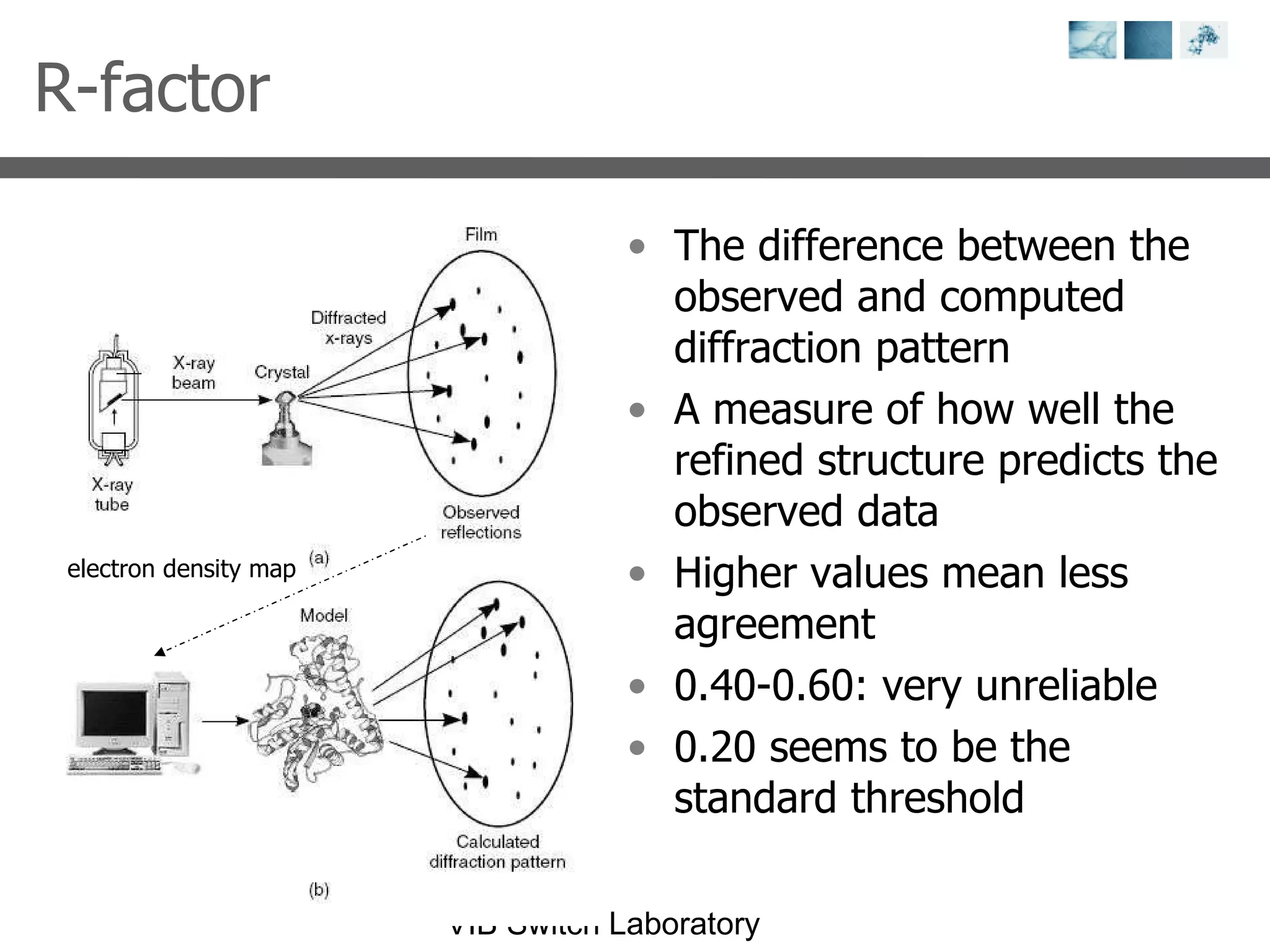
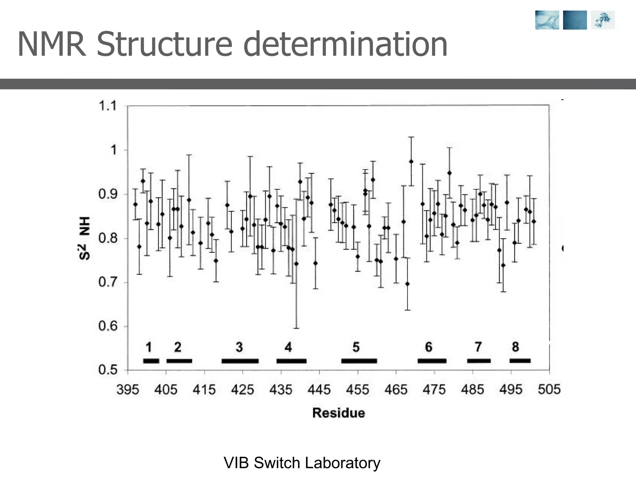
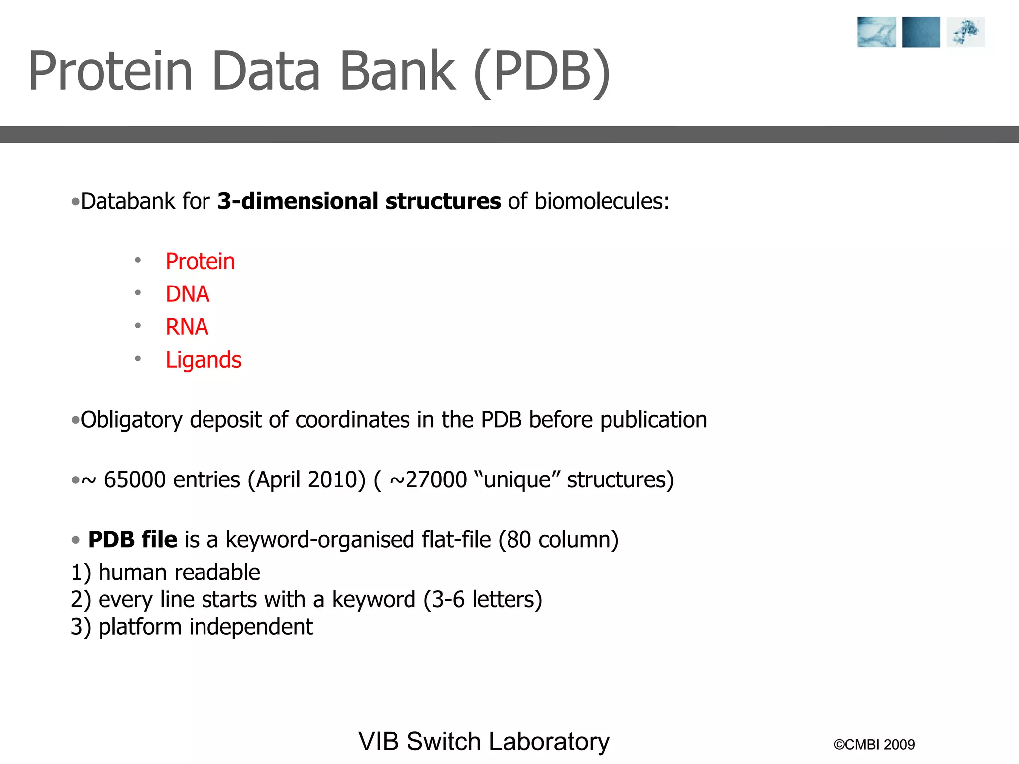
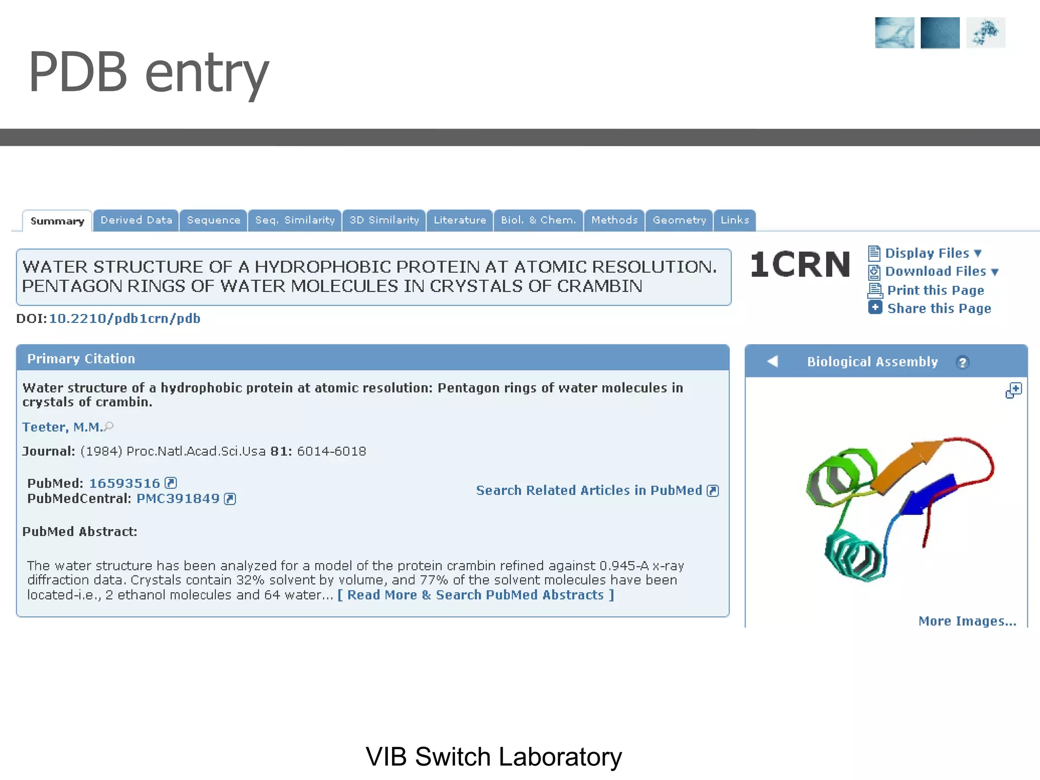
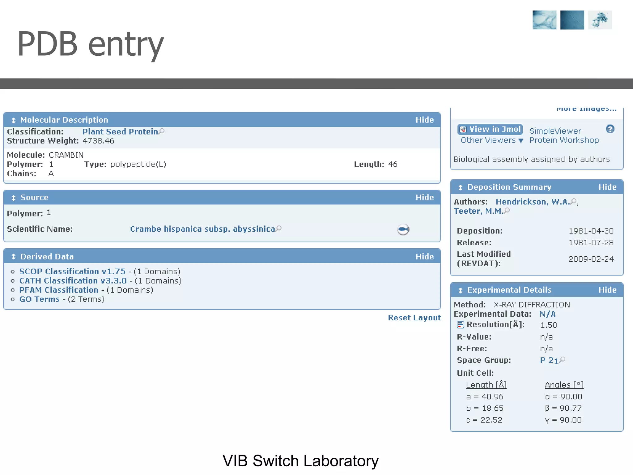
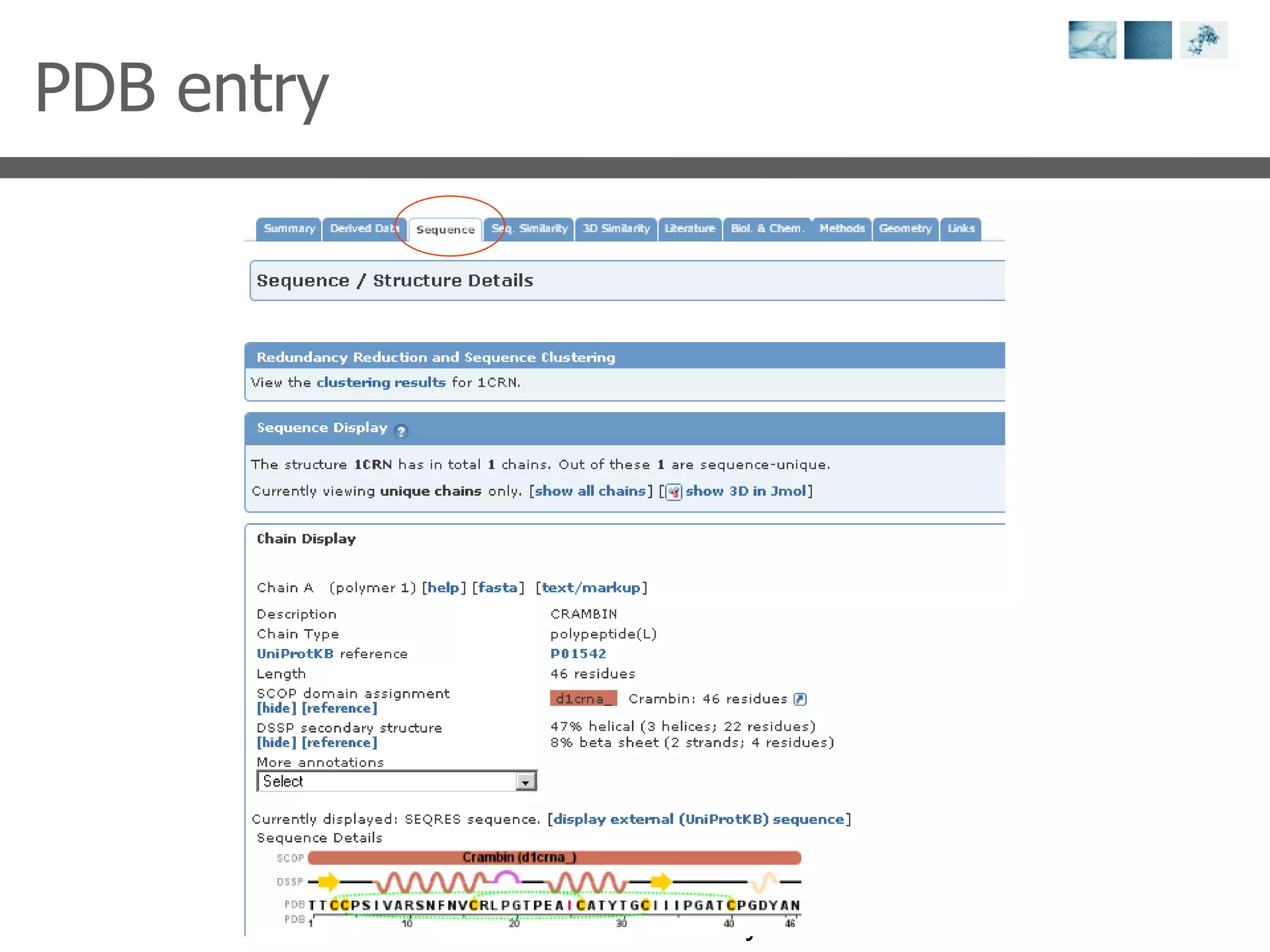
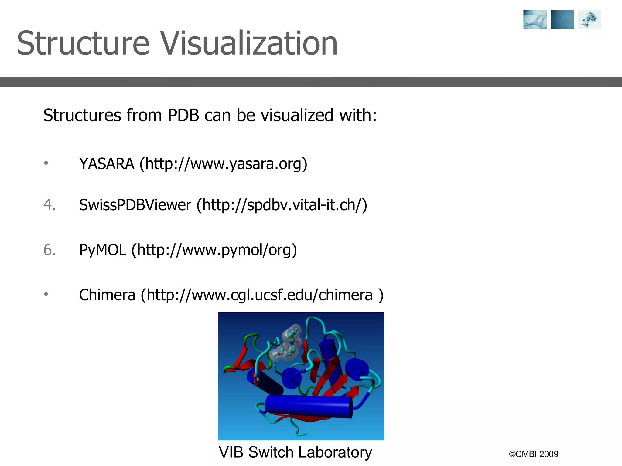
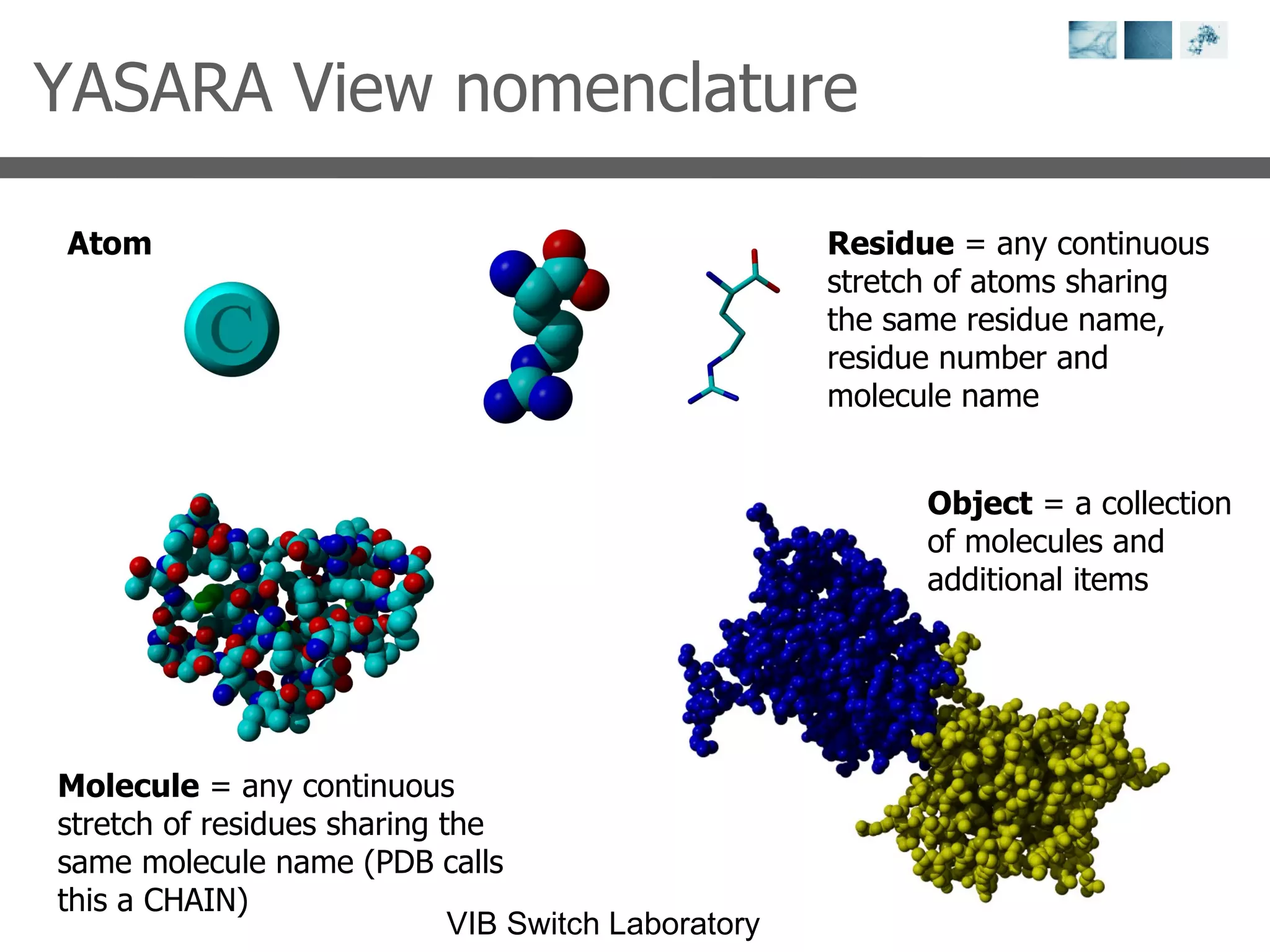
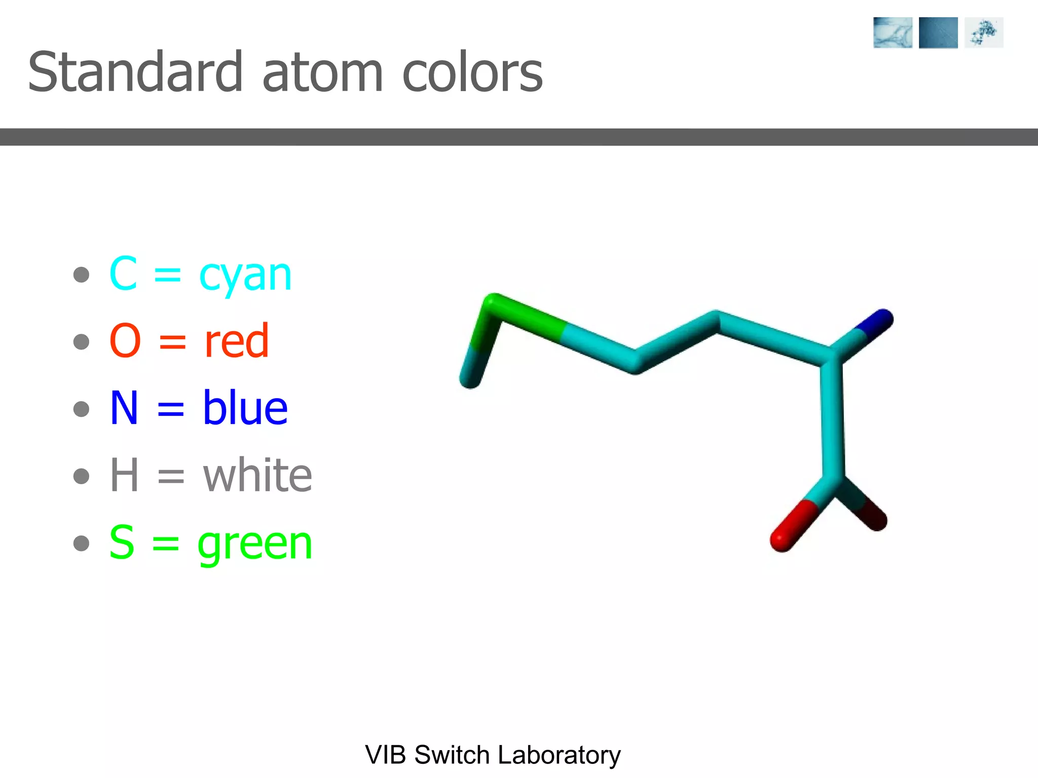


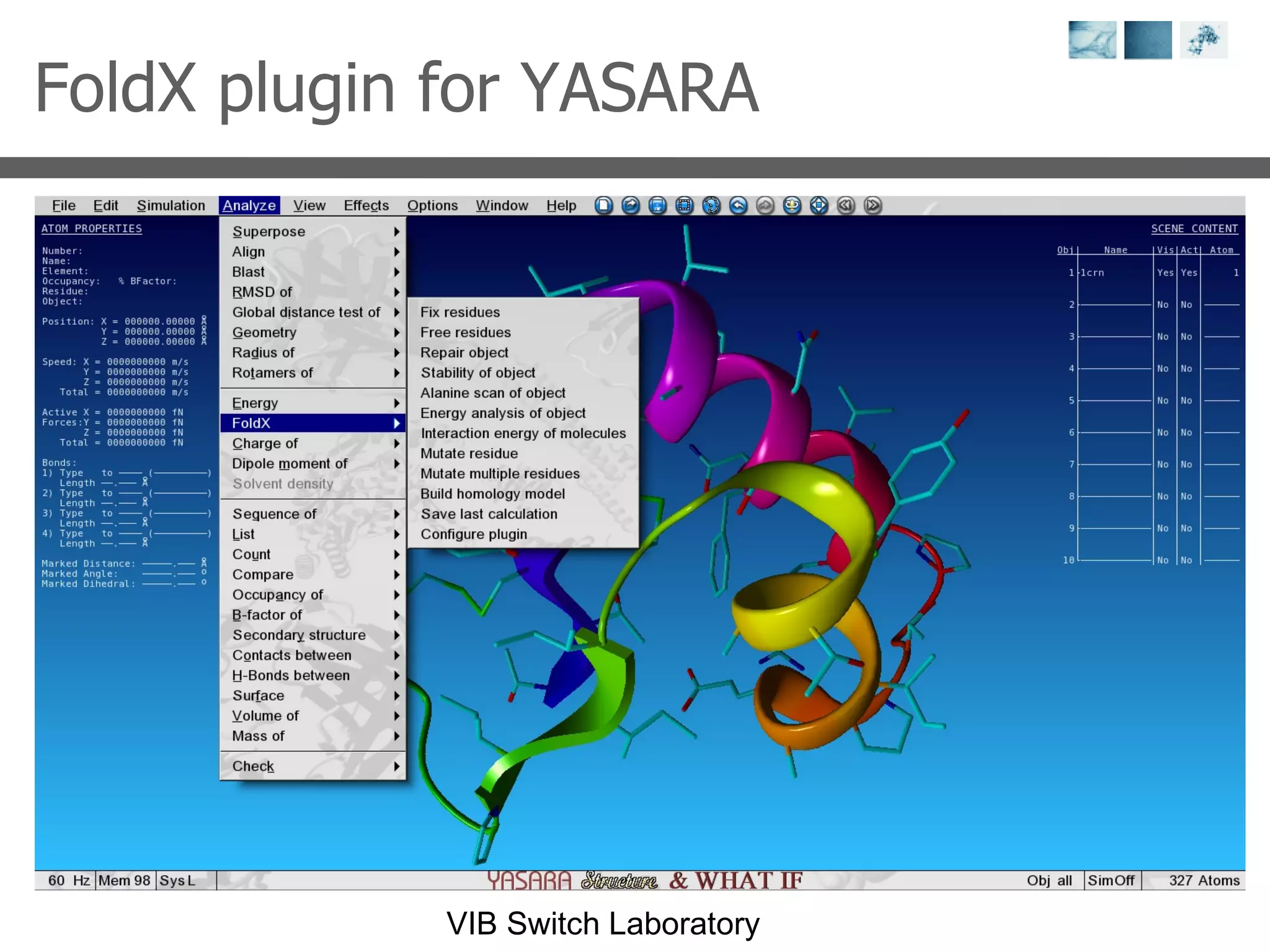

This document provides an overview of protein structure analysis tools and techniques: 1) It describes exploring the Protein Data Bank (PDB) to view and analyze X-ray crystallography and NMR protein structures, comparing similar structures, and using tools like FoldX for in silico mutagenesis and homology modeling. 2) Key concepts covered include PDB file formats, atomic coordinates, B-factors, resolution, RMSD, and the principles of X-ray crystallography, NMR structure determination, and homology modeling. 3) Visualization software like YASARA, SwissPDBViewer and PyMOL are introduced for viewing protein structures from the PDB.


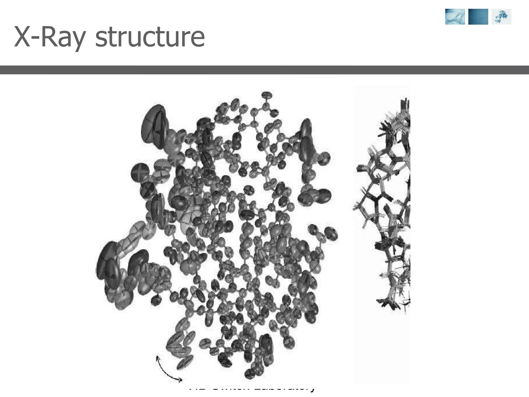
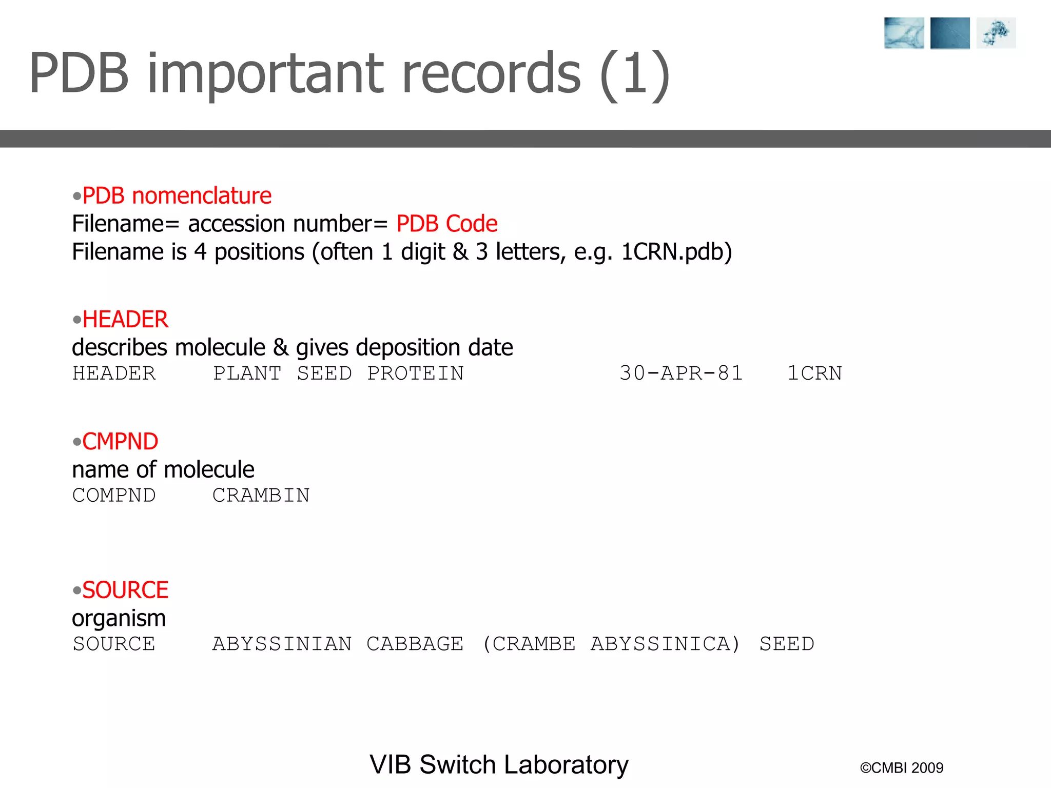
![Coded Agents – with UiPath SDK + LangGraph [Virtual Hands-on Workshop]](https://cdn.slidesharecdn.com/ss_thumbnails/codedagentsdeck-251215155422-5497c599-thumbnail.jpg?width=640&height=640&fit=bounds)


