Downloaded 212 times
![14 of 44
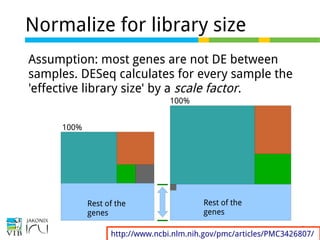
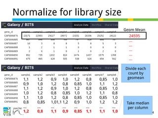
Normalize for library size
DESeq computes a scaling factor for a given sample by computing the median of the ratio, for each gene, of its
read count over its geometric mean across all samples. It then uses the assumption that most genes are not DE
and uses this median of ratios to obtain the scaling factor associated with this sample.
Original library size * scale factor = effective library size
DESeq will multiply original counts by the sample
scaling factor.
DESeq: This normalization method [14] is included in the DESeq Bioconductor package (ver-
sion 1.6.0) [14] and is based on the hypothesis that most genes are not DE. A DESeq scaling
factor for a given lane is computed as the median of the ratio, for each gene, of its read count
over its geometric mean across all lanes. The underlying idea is that non-DE genes should have
similar read counts across samples, leading to a ratio of 1. Assuming most genes are not DE, the
median of this ratio for the lane provides an estimate of the correction factor that should be
applied to all read counts of this lane to fulfill the hypothesis
http://www.ncbi.nlm.nih.gov/pmc/articles/PMC3426807/](https://image.slidesharecdn.com/5-140430070017-phpapp01/85/Part-5-of-RNA-seq-for-DE-analysis-Detecting-differential-expression-14-320.jpg)
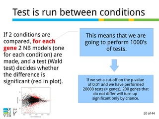
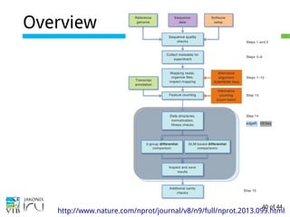

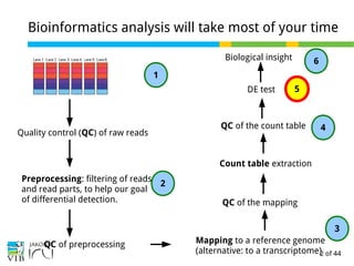
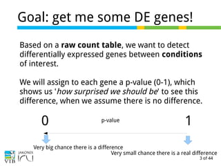
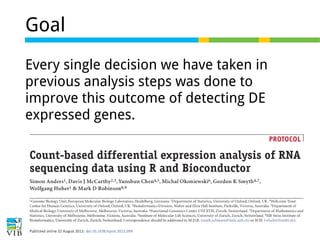
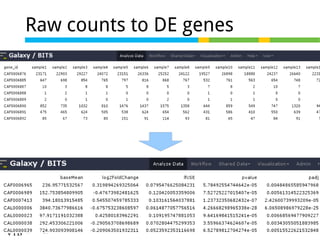
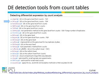
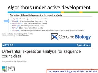
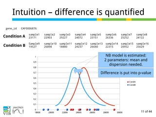
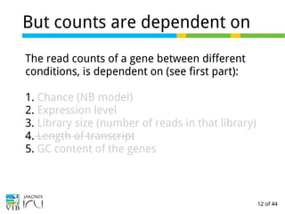
This presentation outlines the steps for bioinformatics analysis of RNA-seq data, focusing on the detection of differentially expressed (DE) genes between conditions. It emphasizes the importance of quality control, normalization, dispersion estimation, and multiple testing corrections to achieve reliable results. Key tools and methodologies such as DESeq2 and independent filtering are discussed for effective gene expression analysis.